손글씨 숫자 인식(MNIST)
- 이 예제는 수학 기초, 모델 설계·학습, 최적화, 배포를 모두 포함합니다.
1. 데이터 준비 (수학 기초 활용)
-
MNIST 데이터셋: 28×28 픽셀의 손글씨 숫자 이미지 (0~9)
-
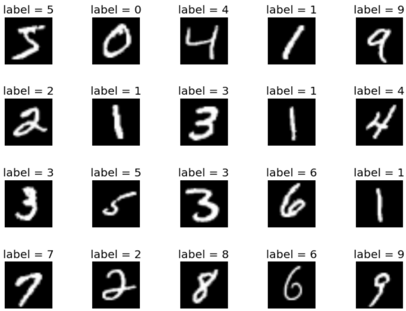
MNIST를 간단히 표현하자면, 누군가가 개발한 인공지능 신경망을 평가하기 위한 자료의 집합 이라고 할 수도 있겠다. 실제로 MNIST는 손글씨 숫자 이미지 집합이다.
-
이는 MNIST Data set의 일부이다. 위와 같은 28x28픽셀 사이즈의 손글씨 사진들이 훈련이미지 60,000장, 시험이미지 10,000장 가량 모여있는 집합이 MNIST Data set이다.
-
각각의 이미지에는 위 그림처럼 정답을 가르키는 label이 달려있다.
-
-
선형대수: 이미지 → 행렬, CNN 합성곱 연산 이해
-
확률: Softmax로 각 숫자 확률 계산
-
미적분: 경사하강법으로 파라미터 업데이트
from torchvision import datasets, transforms

transform = transforms.Compose([transforms.ToTensor()])
train_data = datasets.MNIST(root='./data', train=True, download=True, transform=transform)
test_data = datasets.MNIST(root='./data', train=False, download=True, transform=transform)
2. 모델 설계·학습 (ML/DL 구조)
-
CNN 모델로 이미지 분류
-
손실 함수: CrossEntropyLoss
-
옵티마이저: Adam
import torch.nn as nn

class SimpleCNN(nn.Module):
    def __init__(self):
        super(SimpleCNN, self).__init__()
        self.conv1 = nn.Conv2d(1, 32, 3, 1)
        self.fc1 = nn.Linear(5408, 128)
        self.fc2 = nn.Linear(128, 10)

    def forward(self, x):
        x = self.conv1(x)
        x = nn.functional.relu(x)
        x = nn.Flatten()(x)
        x = self.fc1(x)
        x = nn.functional.relu(x)
        x = self.fc2(x)
        return x
3. 모델 최적화
-
Quantization: 32bit → 8bit로 변환
-
Pruning: 중요도 낮은 가중치 제거
import torch
model = SimpleCNN()
model.eval()
quantized_model = torch.quantization.quantize_dynamic(model, {nn.Linear}, dtype=torch.qint8)
4. 배포 (FastAPI + ONNX)
-
ONNX 변환 후 FastAPI로 REST API 제공
-
서버 서빙:
/predict엔드포인트에서 이미지 업로드 → 숫자 예측
import onnx
torch.onnx.export(quantized_model, torch.randn(1, 1, 28, 28), "mnist_model.onnx")

# FastAPI 예시
from fastapi import FastAPI, File
import numpy as np
import onnxruntime as ort

app = FastAPI()
session = ort.InferenceSession("mnist_model.onnx")

@app.post("/predict")
def predict(file: bytes = File(...)):
    img = np.frombuffer(file, dtype=np.uint8).reshape(1, 1, 28, 28).astype(np.float32)
    outputs = session.run(None, {"input": img})
    pred = np.argmax(outputs[0])
    return {"prediction": int(pred)}
이 예제에서 테스트되는 것
1. 수학 기초: CNN 합성곱(행렬 곱), Softmax 확률, 경사하강법
2. ML/DL 구조: 데이터 → 모델 → 학습 → 추론
3. 모델 최적화: Quantization, Pruning
4. 배포 구조: ONNX 변환, FastAPI API 서빙
한 번에 실행 가능한 전체 워크플로우
1단계: 환경 설정
1.1 Python & 필수 라이브러리 설치
아래 명령어를 터미널(또는 Colab 셀)에 입력하세요.
# 가상환경 생성 (선택)
python -m venv ai_env
source ai_env/bin/activate  # Mac/Linux
ai_env\Scripts\activate     # Windows

# 필수 라이브러리 설치
pip install torch torchvision torchaudio
pip install onnx onnxruntime
pip install fastapi uvicorn
pip install pillow numpy
💡 설명
torch,torchvision: 모델 학습onnx,onnxruntime: 모델 변환 및 실행fastapi,uvicorn: API 서버pillow,numpy: 이미지 처리
2단계: 데이터 준비
from torchvision import datasets, transforms
from torch.utils.data import DataLoader

# 데이터 전처리: Tensor 변환 + 정규화
transform = transforms.Compose([
    transforms.ToTensor(),
    transforms.Normalize((0.1307,), (0.3081,))
])

# 학습/테스트 데이터셋 다운로드
train_dataset = datasets.MNIST(root='./data', train=True, download=True, transform=transform)
test_dataset = datasets.MNIST(root='./data', train=False, download=True, transform=transform)

# DataLoader 생성
train_loader = DataLoader(train_dataset, batch_size=64, shuffle=True)
test_loader = DataLoader(test_dataset, batch_size=1000, shuffle=False)
3단계: 모델 설계 & 학습
import torch
import torch.nn as nn
import torch.optim as optim
import torch.nn.functional as F

# CNN 모델 정의
class SimpleCNN(nn.Module):
    def __init__(self):
        super(SimpleCNN, self).__init__()
        self.conv1 = nn.Conv2d(1, 32, 3, 1)
        self.fc1 = nn.Linear(5408, 128)
        self.fc2 = nn.Linear(128, 10)

    def forward(self, x):
        x = self.conv1(x)
        x = F.relu(x)
        x = torch.flatten(x, 1)
        x = self.fc1(x)
        x = F.relu(x)
        x = self.fc2(x)
        return x

# 모델, 손실함수, 옵티마이저 설정
device = torch.device("cuda" if torch.cuda.is_available() else "cpu")
model = SimpleCNN().to(device)
criterion = nn.CrossEntropyLoss()
optimizer = optim.Adam(model.parameters(), lr=0.001)

# 학습 함수
def train_model(epochs=1):
    model.train()
    for epoch in range(epochs):
        for data, target in train_loader:
            data, target = data.to(device), target.to(device)
            optimizer.zero_grad()
            output = model(data)
            loss = criterion(output, target)
            loss.backward()
            optimizer.step()
        print(f"Epoch {epoch+1}, Loss: {loss.item():.4f}")

train_model(epochs=2)  # 빠른 테스트를 위해 2 epoch만
4단계: 모델 최적화 (Quantization)
# 동적 양자화 적용
quantized_model = torch.quantization.quantize_dynamic(
    model, {nn.Linear}, dtype=torch.qint8
)

# 저장
torch.save(quantized_model.state_dict(), "mnist_quantized.pth")
5단계: ONNX 변환
dummy_input = torch.randn(1, 1, 28, 28, device=device)
torch.onnx.export(
    quantized_model,
    dummy_input.cpu(),
    "mnist_model.onnx",
    input_names=["input"],
    output_names=["output"],
    dynamic_axes={"input": {0: "batch_size"}, "output": {0: "batch_size"}}
)
print("ONNX 모델 저장 완료")
6단계: FastAPI 배포
app.py파일 생성
from fastapi import FastAPI, File, UploadFile
import numpy as np
import onnxruntime as ort
from PIL import Image

app = FastAPI()
session = ort.InferenceSession("mnist_model.onnx")

@app.post("/predict")
async def predict(file: UploadFile = File(...)):
    image = Image.open(file.file).convert("L").resize((28, 28))
    img_array = np.array(image).astype(np.float32) / 255.0
    img_array = (img_array - 0.1307) / 0.3081
    img_array = img_array.reshape(1, 1, 28, 28)

    outputs = session.run(None, {"input": img_array})
    pred = int(np.argmax(outputs[0]))
    return {"prediction": pred}
7단계: 서버 실행
uvicorn app:app --reload- 브라우저에서
http://127.0.0.1:8000/docs접속 /predict엔드포인트에서 이미지 업로드 → 예측 결과 확인
8단계: 테스트
curl -X POST "http://127.0.0.1:8000/predict" \
  -F "file=@sample_digit.png"
응답 예시:
{"prediction": 7}진행 순서
-
새 가상환경(venv) 세팅 → 깨진 env 대신 사용
-
필요 패키지 설치
-
mnist_pipeline.ipynb파일 생성 -
Jupyter에서 실행 테스트
1) 새 가상환경 만들기
- PowerShell
# ML 폴더에서 실행
python -m venv venv
venv\Scripts\activate

# pip 최신화
pip install --upgrade pip setuptools wheel
2) 필수 패키지 설치
pip install torch torchvision torchaudio
pip install onnx onnxruntime
pip install fastapi uvicorn
pip install pillow numpy
pip install notebook
3) mnist_pipeline.ipynb 만들기
- 아래 코드를 복사해서 Jupyter Notebook에서 새 파일로 붙여넣고 저장하세요.
# 1. 환경 설정 (이미 설치했으면 건너뛰기)
# !pip install torch torchvision torchaudio
# !pip install onnx onnxruntime
# !pip install fastapi uvicorn
# !pip install pillow numpy

# 2. 데이터 준비
from torchvision import datasets, transforms
from torch.utils.data import DataLoader

transform = transforms.Compose([
    transforms.ToTensor(),
    transforms.Normalize((0.1307,), (0.3081,))
])

train_dataset = datasets.MNIST(root='./data', train=True, download=True, transform=transform)
test_dataset = datasets.MNIST(root='./data', train=False, download=True, transform=transform)

train_loader = DataLoader(train_dataset, batch_size=64, shuffle=True)
test_loader = DataLoader(test_dataset, batch_size=1000, shuffle=False)

# 3. 모델 설계 & 학습
import torch
import torch.nn as nn
import torch.optim as optim
import torch.nn.functional as F

class SimpleCNN(nn.Module):
    def __init__(self):
        super(SimpleCNN, self).__init__()
        self.conv1 = nn.Conv2d(1, 32, 3, 1)
        self.fc1 = nn.Linear(5408, 128)
        self.fc2 = nn.Linear(128, 10)

    def forward(self, x):
        x = self.conv1(x)
        x = F.relu(x)
        x = torch.flatten(x, 1)
        x = self.fc1(x)
        x = F.relu(x)
        x = self.fc2(x)
        return x

device = torch.device("cuda" if torch.cuda.is_available() else "cpu")
model = SimpleCNN().to(device)
criterion = nn.CrossEntropyLoss()
optimizer = optim.Adam(model.parameters(), lr=0.001)

def train_model(epochs=1):
    model.train()
    for epoch in range(epochs):
        for data, target in train_loader:
            data, target = data.to(device), target.to(device)
            optimizer.zero_grad()
            output = model(data)
            loss = criterion(output, target)
            loss.backward()
            optimizer.step()
        print(f"Epoch {epoch+1}, Loss: {loss.item():.4f}")

train_model(epochs=2)

# 4. 모델 최적화
quantized_model = torch.quantization.quantize_dynamic(
    model, {nn.Linear}, dtype=torch.qint8
)
torch.save(quantized_model.state_dict(), "mnist_quantized.pth")

# 5. ONNX 변환
dummy_input = torch.randn(1, 1, 28, 28, device=device)
torch.onnx.export(
    quantized_model,
    dummy_input.cpu(),
    "mnist_model.onnx",
    input_names=["input"],
    output_names=["output"],
    dynamic_axes={"input": {0: "batch_size"}, "output": {0: "batch_size"}}
)
print("ONNX 모델 저장 완료")

# 6. FastAPI 서버
from fastapi import FastAPI, File, UploadFile
import numpy as np
import onnxruntime as ort
from PIL import Image

app = FastAPI()
session = ort.InferenceSession("mnist_model.onnx")

@app.post("/predict")
async def predict(file: UploadFile = File(...)):
    image = Image.open(file.file).convert("L").resize((28, 28))
    img_array = np.array(image).astype(np.float32) / 255.0
    img_array = (img_array - 0.1307) / 0.3081
    img_array = img_array.reshape(1, 1, 28, 28)

    outputs = session.run(None, {"input": img_array})
    pred = int(np.argmax(outputs[0]))
    return {"prediction": pred}

# Jupyter에서 서버 실행
# !uvicorn app:app --reload --port 8000
4) 실행
venv\Scripts\activate
jupyter notebook-
mnist_pipeline.ipynb열기 -
셀 순서대로 실행
-
마지막 셀에서 FastAPI 서버 실행 후, 브라우저에서
http://127.0.0.1:8000/docs접속 → 이미지 업로드 테스트
확장판
# =========================================
# 1. 환경 설정 (필요 패키지 설치)
# =========================================
# !를 붙이면 Jupyter Notebook에서 터미널 명령어 실행 가능
# 아래 명령은 현재 커널의 Python 환경에 패키지를 설치합니다.
!pip install torch torchvision torchaudio   # PyTorch 및 데이터셋 관련 라이브러리
!pip install onnx onnxruntime               # ONNX 변환 및 실행 라이브러리
!pip install fastapi uvicorn                # FastAPI 서버 및 실행기
!pip install pillow numpy matplotlib        # 이미지 처리(Pillow), 수치연산(Numpy), 시각화(Matplotlib)

# =========================================
# 2. 커널 환경 확인
# =========================================
# 현재 Notebook이 어떤 Python 환경을 쓰는지 확인
# 설치한 패키지가 이 환경에 들어가야 정상 동작합니다.
import sys
print("현재 Python 실행 경로:", sys.executable)

# =========================================
# 3. 데이터 준비
# =========================================
# MNIST 데이터셋 다운로드 및 전처리
# transforms.Normalize: 픽셀값을 평균 0.1307, 표준편차 0.3081로 정규화
from torchvision import datasets, transforms
from torch.utils.data import DataLoader

transform = transforms.Compose([
    transforms.ToTensor(),
    transforms.Normalize((0.1307,), (0.3081,))
])

# 학습용(train)과 테스트용(test) 데이터셋 로드
train_dataset = datasets.MNIST(root='./data', train=True, download=True, transform=transform)
test_dataset = datasets.MNIST(root='./data', train=False, download=True, transform=transform)

# DataLoader: 배치 단위로 데이터를 불러오는 도구
train_loader = DataLoader(train_dataset, batch_size=64, shuffle=True)
test_loader = DataLoader(test_dataset, batch_size=1000, shuffle=False)

# =========================================
# 4. 모델 설계
# =========================================
# 간단한 CNN 모델 정의
# Conv2d → ReLU → Flatten → FC → ReLU → FC → 출력
import torch
import torch.nn as nn
import torch.nn.functional as F

class SimpleCNN(nn.Module):
    def __init__(self):
        super(SimpleCNN, self).__init__()
        self.conv1 = nn.Conv2d(1, 32, 3, 1)   # 입력 채널 1, 출력 채널 32, 커널 크기 3x3
        self.fc1 = nn.Linear(21632, 128)      # Conv2d 출력 크기에 맞춰 입력 크기 설정
        self.fc2 = nn.Linear(128, 10)         # 10개의 클래스(MNIST 숫자 0~9)

    def forward(self, x):
        x = self.conv1(x)
        x = F.relu(x)
        x = torch.flatten(x, 1)  # 배치 차원 제외하고 평탄화
        x = self.fc1(x)
        x = F.relu(x)
        x = self.fc2(x)
        return x

# =========================================
# 5. 학습 준비
# =========================================
# GPU 사용 가능하면 GPU로, 아니면 CPU로 설정
import torch.optim as optim

device = torch.device("cuda" if torch.cuda.is_available() else "cpu")
model = SimpleCNN().to(device)
criterion = nn.CrossEntropyLoss()  # 분류 문제 손실 함수
optimizer = optim.Adam(model.parameters(), lr=0.001)  # Adam 옵티마이저

# =========================================
# 6. 학습 (Accuracy 출력)
# =========================================
# 학습 과정에서 Loss와 Accuracy를 출력하여 성능 확인
def train_model(epochs=1):
    model.train()  # 학습 모드
    for epoch in range(epochs):
        correct = 0
        total = 0
        for data, target in train_loader:
            data, target = data.to(device), target.to(device)
            optimizer.zero_grad()
            output = model(data)
            loss = criterion(output, target)
            loss.backward()
            optimizer.step()

            # 예측값 계산
            pred = output.argmax(dim=1)
            correct += pred.eq(target).sum().item()
            total += target.size(0)

        acc = 100. * correct / total
        print(f"Epoch {epoch+1}, Loss: {loss.item():.4f}, Accuracy: {acc:.2f}%")

train_model(epochs=2)

# =========================================
# 7. 테스트 평가
# =========================================
# 학습된 모델을 테스트 데이터로 평가
def test_model():
    model.eval()  # 평가 모드
    correct = 0
    total = 0
    with torch.no_grad():  # 평가 시에는 gradient 계산 안 함
        for data, target in test_loader:
            data, target = data.to(device), target.to(device)
            output = model(data)
            pred = output.argmax(dim=1)
            correct += pred.eq(target).sum().item()
            total += target.size(0)
    acc = 100. * correct / total
    print(f"Test Accuracy: {acc:.2f}%")

test_model()

# =========================================
# 8. 예측 시각화
# =========================================
# 테스트 데이터 일부를 시각화하여 예측값과 실제값 비교
import matplotlib.pyplot as plt

def show_predictions(n=5):
    model.eval()
    images, labels = next(iter(test_loader))
    images, labels = images.to(device), labels.to(device)
    outputs = model(images)
    preds = outputs.argmax(dim=1)

    plt.figure(figsize=(10, 2))
    for i in range(n):
        plt.subplot(1, n, i+1)
        plt.imshow(images[i].cpu().squeeze(), cmap='gray')
        plt.title(f"P:{preds[i].item()} / T:{labels[i].item()}")
        plt.axis('off')
    plt.show()

show_predictions(5)

# =========================================
# 9. FastAPI 테스트용 이미지 생성
# =========================================
# FastAPI API 테스트를 위해 샘플 이미지 저장
from torchvision.utils import save_image

img, label = test_dataset[0]
save_image(img, f"sample_{label}.png")
print(f"Saved sample image with label {label}")

# =========================================
# 10. 모델 최적화 (Quantization)
# =========================================
# Linear 레이어를 동적 양자화하여 모델 크기와 추론 속도 개선
quantized_model = torch.quantization.quantize_dynamic(
    model, {nn.Linear}, dtype=torch.qint8
)
torch.save(quantized_model.state_dict(), "mnist_quantized.pth")

# =========================================
# 11. ONNX 변환
# =========================================
# PyTorch 모델을 ONNX 포맷으로 변환하여 다양한 환경에서 실행 가능하게 함
dummy_input = torch.randn(1, 1, 28, 28, device=device)
torch.onnx.export(
    quantized_model,
    dummy_input.cpu(),
    "mnist_model.onnx",
    input_names=["input"],
    output_names=["output"],
    dynamic_axes={"input": {0: "batch_size"}, "output": {0: "batch_size"}}
)
print("ONNX 모델 저장 완료")

# =========================================
# 12. FastAPI 서버
# =========================================
# ONNX 모델을 로드하여 API로 예측 서비스 제공
from fastapi import FastAPI, File, UploadFile
import numpy as np
import onnxruntime as ort
from PIL import Image

app = FastAPI()
session = ort.InferenceSession("mnist_model.onnx")

@app.post("/predict")
async def predict(file: UploadFile = File(...)):
    # 업로드된 이미지를 흑백으로 변환하고 28x28로 리사이즈
    image = Image.open(file.file).convert("L").resize((28, 28))
    img_array = np.array(image).astype(np.float32) / 255.0
    img_array = (img_array - 0.1307) / 0.3081  # MNIST 정규화
    img_array = img_array.reshape(1, 1, 28, 28)

    # ONNX 모델로 추론
    outputs = session.run(None, {"input": img_array})
    pred = int(np.argmax(outputs[0]))
    return {"prediction": pred}

# =========================================
# 13. FastAPI 실행 (Jupyter에서)
# =========================================
# 주석 해제 후 실행하면 서버가 켜집니다.
# 브라우저에서 http://127.0.0.1:8000/docs 접속 → /predict 엔드포인트 테스트
# !uvicorn app:app --reload --port 8000
학습 중간 진행률과 배치별 성능
- 배치 단위 로그 출력
train_loader에서 몇 번째 배치인지 출력- 진행률 계산:
(현재 배치 / 전체 배치) * 100
- 미니 배치 평균 Loss 출력
- 일정 간격(예: 100 step마다)만 출력해서 로그 과다 방지
- 테스트 평가도 중간 로그
- 테스트 데이터셋이 크면 중간에 Accuracy를 찍어줌
def train_model(epochs=1, log_interval=100):
    model.train()
    for epoch in range(epochs):
        correct = 0
        total = 0
        for batch_idx, (data, target) in enumerate(train_loader):
            data, target = data.to(device), target.to(device)
            optimizer.zero_grad()
            output = model(data)
            loss = criterion(output, target)
            loss.backward()
            optimizer.step()

            # 예측값 계산
            pred = output.argmax(dim=1)
            correct += pred.eq(target).sum().item()
            total += target.size(0)

            # 일정 간격마다 로그 출력
            if batch_idx % log_interval == 0:
                progress = 100. * batch_idx / len(train_loader)
                batch_acc = 100. * pred.eq(target).sum().item() / target.size(0)
                print(f"Epoch {epoch+1} [{batch_idx}/{len(train_loader)} "
                      f"({progress:.0f}%)]\tLoss: {loss.item():.4f}\tBatch Acc: {batch_acc:.2f}%")

        # Epoch 종료 후 전체 Accuracy 출력
        acc = 100. * correct / total
        print(f"==> Epoch {epoch+1} 완료 | Loss: {loss.item():.4f} | Accuracy: {acc:.2f}%\n")
def test_model(log_interval=5):
model.eval()
correct = 0
total = 0
with torch.no_grad():
for batch_idx, (data, target) in enumerate(test_loader):
data, target = data.to(device), target.to(device)
output = model(data)
pred = output.argmax(dim=1)
correct += pred.eq(target).sum().item()
total += target.size(0)
# 일정 간격마다 로그 출력
if batch_idx % log_interval == 0:
progress = 100. * batch_idx / len(test_loader)
batch_acc = 100. * pred.eq(target).sum().item() / target.size(0)
print(f"Test Batch {batch_idx}/{len(test_loader)} "
f"({progress:.0f}%)]\tBatch Acc: {batch_acc:.2f}%")
acc = 100. * correct / total
print(f"==> Test Accuracy: {acc:.2f}%\n")train_model(epochs=2, log_interval=200)
test_model(log_interval=2)출력 예시
Epoch 1 [0/938 (0%)]    Loss: 2.3026    Batch Acc: 9.38%
Epoch 1 [200/938 (21%)] Loss: 0.4567    Batch Acc: 87.50%
Epoch 1 [400/938 (43%)] Loss: 0.3214    Batch Acc: 90.62%
...
==> Epoch 1 완료 | Loss: 0.1234 | Accuracy: 96.45%

Test Batch 0/10 (0%)]   Batch Acc: 98.00%
Test Batch 2/10 (20%)]  Batch Acc: 97.50%
...
==> Test Accuracy: 97.85%