
📦 Lab: IMDB Document Classification
# Convert IMDB dataset in the keras package to be suitable for torch
(imdb_seq_train, imdb_seq_test) = load_sequential(root='data/IMDB')

padded_sample   = np.asarray(imdb_seq_train.tensors[0][0])
sample_review   = padded_sample[padded_sample > 0][:12]
sample_review[:12]

load_sequential() 함수는 IMDB 데이터셋을 불러올 때 각 리뷰를 시퀀스로 표현하며, 이 시퀀스는 최대 500개의 단어로 제한된 패딩(padded)된 형태이다.
즉, 긴 리뷰는 마지막 500단어만 사용되고, 짧은 리뷰는 앞에 0으로 패딩된다.
lookup = load_lookup(root='data/IMDB')
' '.join(lookup[i] for i in sample_review)
대부분의 리뷰가 매우 짧기 때문에, 이러한 특징 행렬(feature matrix)은 98% 이상이 0으로 채워져 있다.
# Set data
max_num_workers = 10

(imdb_train, imdb_test) = load_tensor(root='data/IMDB')

imdb_dm = SimpleDataModule(imdb_train,
                           imdb_test,
                           validation=2000,
                           num_workers=min(6, max_num_workers),
                           batch_size=512)
load_tensor()은 IMDB 데이터를 불러오는 함수로, 희소 텐서(sparse tensor) 형식으로 데이터를 로드하여 PyTorch에서 바로 사용할 수 있도록 구성한다.
- BoW(Bag-of-Words) 형식의 데이터처럼 대부분이 0으로 이루어진 텍스트 데이터를 효율적으로 표현할 수 있음
- torch의
TensorDataset형태로 반환되어,SimpleDataModule등에 바로 활용 가능 validation인자를 통해 검증 세트를 분리할 수 있음
즉, 희소한 텍스트 데이터를 torch가 다룰 수 있는 구조로 변환해주는 전처리 역할을 한다.
# Use a two-layer model for our first model.
class IMDBModel(nn.Module):
    def __init__(self, input_size):
        super(IMDBModel, self).__init__()
        self.dense1     = nn.Linear(input_size, 16)
        self.activation = nn.ReLU()
        self.dense2     = nn.Linear(16, 16)
        self.output     = nn.Linear(16, 1)

    def forward(self, x):
        val = x
        for _map in [self.dense1,
                     self.activation,
                     self.dense2,
                     self.activation,
                     self.output]:
            val = _map(val)
        return torch.flatten(val)
# Instantiate our model
imdb_model = IMDBModel(imdb_test.tensors[0].size()[1])
# Show model summary
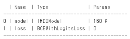
summary(imdb_model,
input_size=imdb_test.tensors[0].size(),
col_names=['input_size', 'output_size', 'num_params'])

# Use a smaller learning rate for the data
imdb_optimizer = RMSprop(imdb_model.parameters(), lr=0.001)

# Define the binary classification module
imdb_module = SimpleModule.binary_classification(imdb_model,
                                                  optimizer=imdb_optimizer)

# Set up logger and trainer
imdb_logger = CSVLogger('logs', name='IMDB')
imdb_trainer = Trainer(deterministic=True,
                       max_epochs=30,
                       logger=imdb_logger,
                       callbacks=[ErrorTracker()])

# Train the model
imdb_trainer.fit(imdb_module, datamodule=imdb_dm)
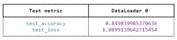
# Evaluate the test error
test_results = imdb_trainer.test(imdb_module,
                                  datamodule=imdb_dm)

test_results
# Fit a lasso logistic regression model using LogisticRegression() from sklearn
((X_train, Y_train),
 (X_valid, Y_valid),
 (X_test, Y_test)) = load_sparse(validation=2000,
                                 random_state=0,
                                 root='data/IMDB')

lam_max   = np.abs(X_train.T * (Y_train - Y_train.mean())).max()
lam_val   = lam_max * np.exp(np.linspace(np.log(1), np.log(1e-4), 50))

logit     = LogisticRegression(penalty='l1',
                               C=1/lam_max,
                               solver='liblinear',
                               warm_start=True,
                               fit_intercept=True)

coefs     = []
intercepts = []
for l in lam_val:
    logit.C = 1 / l
    logit.fit(X_train, Y_train)
    coefs.append(logit.coef_.copy())
    intercepts.append(logit.intercept_)

coefs      = np.squeeze(coefs)
intercepts = np.squeeze(intercepts)
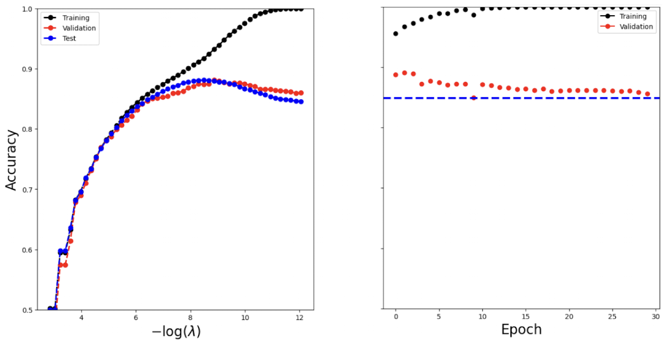
# Make a plot to compare our neural network results with the lasso
%%capture
fig, axes = subplots(1, 2, figsize=(16, 8), sharey=True)

for ((X_, Y_), data_, color) in zip(
    [(X_train, Y_train), (X_valid, Y_valid), (X_test, Y_test)],
    ['Training', 'Validation', 'Test'],
    ['black', 'red', 'blue']
):
    linpred_ = X_ * coefs.T + intercepts[None, :]
    label_ = np.array(linpred_ > 0)
    accuracy_ = np.array([np.mean(Y_ == l) for l in label_.T])

    axes[0].plot(
        -np.log(lam_val / X_train.shape[0]),
        accuracy_,
        '.--',
        color=color,
        linewidth=2,
        label=data_
    )

axes[0].legend()
axes[0].set_xlabel(r'$-\log(\lambda)$', fontsize=20)
axes[0].set_ylabel('Accuracy', fontsize=20)
# Read and plot IMDB results
imdb_results = pd.read_csv(imdb_logger.experiment.metrics_file_path)

summary_plot(
    imdb_results,
    axes[1],
    col='accuracy',
    ylabel='Accuracy'
)

axes[1].set_xticks(np.linspace(0, 30, 7).astype(int))
axes[1].set_ylabel('Accuracy', fontsize=20)
axes[1].set_xlabel('Epoch', fontsize=20)
axes[1].set_ylim([0.5, 1])
axes[1].axhline(
    test_results[0]['test_accuracy'],
    color='blue',
    linestyle='--',
    linewidth=3
)

fig

# Cleanup
del(imdb_model, imdb_trainer, imdb_logger,
    imdb_dm, imdb_train, imdb_test)
📦 Lab: RNN for Document Classification
# Fit a simple LSTM RNN for sentiment prediction
imdb_seq_dm = SimpleDataModule(
imdb_seq_train,
imdb_seq_test,
validation=2000,
batch_size=300,
num_workers=min(6, max_num_workers)
)
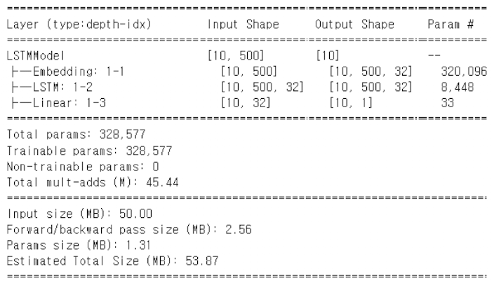
class LSTMModel(nn.Module):
def __init__(self, input_size):
super(LSTMModel, self).__init__()
self.embedding = nn.Embedding(input_size, 32)
self.lstm = nn.LSTM(
input_size=32,
hidden_size=32,
batch_first=True
)
self.dense = nn.Linear(32, 1)
def forward(self, x):
val, (h_n, c_n) = self.lstm(self.embedding(x))
return torch.flatten(self.dense(val[:, -1]))nn.Embedding(10003, 32)의 경우 파라미터 수는: 임베딩 행렬의 크기
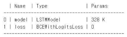
lstm_model = LSTMModel(X_test.shape[-1])

summary(
    lstm_model,
    input_data=imdb_seq_train.tensors[0][:10],
    col_names=['input_size', 'output_size', 'num_params']
)
lstm_module = SimpleModule.binary_classification(lstm_model)

lstm_logger  = CSVLogger('logs', name='IMDB_LSTM')

lstm_trainer = Trainer(
    deterministic=True,
    max_epochs=20,
    logger=lstm_logger,
    callbacks=[ErrorTracker()]
)

lstm_trainer.fit(
    lstm_module,
    datamodule=imdb_seq_dm
)
 ```
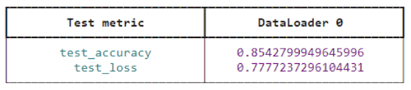
lstm_trainer.test(
lstm_module,
datamodule=imdb_seq_dm
)
```
```
lstm_trainer.test(
lstm_module,
datamodule=imdb_seq_dm
)
```
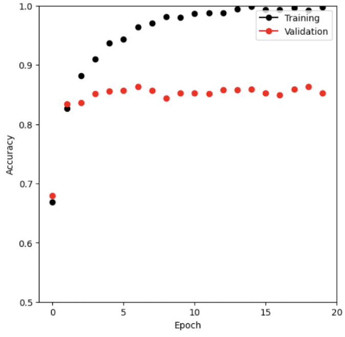
lstm_results = pd.read_csv(lstm_logger.experiment.metrics_file_path)

fig, ax = subplots(1, 1, figsize=(6, 6))
summary_plot(
    lstm_results,
    ax,
    col='accuracy',
    ylabel='Accuracy'
)

ax.set_xticks(np.linspace(0, 20, 5).astype(int))
ax.set_ylabel('Accuracy')
ax.set_ylim([0.5, 1])

# Cleanup
del(
    lstm_model,
    lstm_trainer,
    lstm_logger,
    imdb_seq_dm,
    imdb_seq_train,
    imdb_seq_test
)
📦 Lab: RNN for Time Series Prediction
# Load and standardize the data
NYSE = load_data('NYSE')
cols = ['DJ_return', 'log_volume', 'log_volatility']

X = pd.DataFrame(
    StandardScaler(with_mean=True, with_std=True)
    .fit_transform(NYSE[cols]),
    columns=NYSE[cols].columns,
    index=NYSE.index
)

# Set up the lagged versions of the data
for lag in range(1, 6):
    for col in cols:
        newcol = np.zeros(X.shape[0]) * np.nan
        newcol[lag:] = X[col].values[:-lag]
        X.insert(len(X.columns), f"{col}_{lag}", newcol)

X.insert(len(X.columns), 'train', NYSE['train'])
X = X.dropna()

Y, train = X['log_volume'], X['train']
X = X.drop(columns=['train'] + cols)
X.columns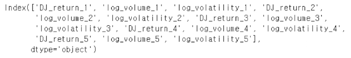
# Fit a simple linear model and compute the R2 on the test data
M = LinearRegression()
M.fit(X[train], Y[train])
M.score(X[~train], Y[~train])
X_day = pd.merge(
    X,
    pd.get_dummies(NYSE['day_of_week']),
    on='date'
)

M.fit(X_day[train], Y[train])
M.score(X_day[~train], Y[~train])
# To fit the RNN, we must reshape the data
ordered_cols = []
for lag in range(5,0,-1):
for col in cols:
ordered_cols.append('{0}_{1}'.format(col, lag))
X = X.reindex(columns=ordered_cols)
X.columns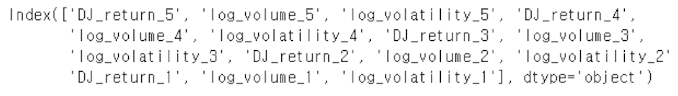
X_rnn = X.to_numpy().reshape((-1, 5, 3))
X_rnn.shape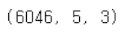
# Define the RNN Model
class NYSEModel(nn.Module):
    def __init__(self):
        super(NYSEModel, self).__init__()
        self.rnn     = nn.RNN(3, 12, batch_first=True)
        self.dense   = nn.Linear(12, 1)
        self.dropout = nn.Dropout(0.1)

    def forward(self, x):
        val, h_n = self.rnn(x)
        val      = self.dense(self.dropout(val[:, -1]))
        return torch.flatten(val)

nyse_model = NYSEModel()
# Form the training dataset
datasets = []
for mask in [train, ~train]:
X_rnn_t = torch.tensor(X_rnn[mask].astype(np.float32))
Y_t = torch.tensor(Y[mask].astype(np.float32))
datasets.append(TensorDataset(X_rnn_t, Y_t))
nyse_train, nyse_test = datasets
# Inspect the summary
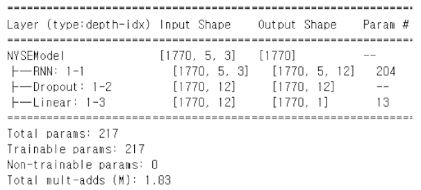
summary(nyse_model,
input_data=X_rnn_t,
col_names=['input_size', 'output_size', 'num_params'])
# Put the two datasets into a data module
nyse_dm = SimpleDataModule(nyse_train,
nyse_test,
num_workers=min(4, max_num_workers),
validation=nyse_test,
batch_size=64)
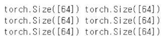
for idx, (x, y) in enumerate(nyse_dm.train_dataloader()):
out = nyse_model(x)
print(y.size(), out.size())
if idx >= 2:
break
nyse_optimizer = RMSprop(nyse_model.parameters(), lr=0.001)
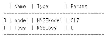
nyse_module = SimpleModule.regression(nyse_model,
optimizer=nyse_optimizer,
metrics={'r2': R2Score()})
nyse_trainer = Trainer(deterministic=True,
max_epochs=200,
callbacks=[ErrorTracker()])
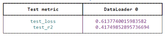
nyse_trainer.fit(nyse_module, datamodule=nyse_dm)
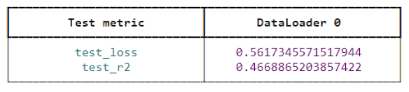
nyse_trainer.test(nyse_module, datamodule=nyse_dm)
# Fit a nonlinear AR model using the feature set X_day
# that includes the day_of_week indicators.
datasets = []
for mask in [train, ~train]:
    X_day_t = torch.tensor(
        np.asarray(X_day[mask]).astype(np.float32)
    )
    Y_t = torch.tensor(
        np.asarray(Y[mask]).astype(np.float32)
    )
    datasets.append(TensorDataset(X_day_t, Y_t))
day_train, day_test = datasets

day_dm = SimpleDataModule(
    day_train,
    day_test,
    num_workers=min(4, max_num_workers),
    validation=day_test,
    batch_size=64
)

# Define AR Model
class NonLinearARModel(nn.Module):
    def __init__(self):
        super(NonLinearARModel, self).__init__()
        self._forward = nn.Sequential(
            nn.Flatten(),
            nn.Linear(20, 32),
            nn.ReLU(),
            nn.Dropout(0.5),
            nn.Linear(32, 1)
        )

    def forward(self, x):
        return torch.flatten(self._forward(x))
nl_model     = NonLinearARModel()

nl_optimizer = RMSprop(nl_model.parameters(), lr=0.001)

nl_module    = SimpleModule.regression(
    nl_model,
    optimizer=nl_optimizer,
    metrics={'r2': R2Score()}
)

nl_trainer   = Trainer(
    deterministic=True,
    max_epochs=20,
    callbacks=[ErrorTracker()]
)

nl_trainer.fit(nl_module, datamodule=day_dm)
nl_trainer.test(nl_module, datamodule=day_dm)

🐾