
기초부터 쌓아가는 머신러닝 #2
2주차 : pandas 라이브러리 기초 실습
- DataFrame 행, 열 선택 및 필터링 복습
import os
import pandas as pd

os.listdir('./drive/MyDrive/machine_learning_data')
> ['friend.csv']

# 데이터 폴더 src 변수 할당
base_src = './drive/MyDrive/machine_learning_data'
# friend.csv 파일 src 변수 할당
friend_src = base_src+"/friend.csv"

# friend.csv 불러오기
df = pd.read_csv(friend_src,encoding='utf-8')
df.head()
>	name	age	job
0	John	20	student
1	Jenny	30	developer
2	Nate	30	teacher
3	Julia	40	dentist
4	Brian	45	manager

# index 2번에 해당하는 row 가져오기
df.iloc[2] # Series 형태로 가져옴
>name       Nate
age          30
job     teacher
Name: 2, dtype: object

# column job에 해당되는 데이터 가져오기(1)
df['job']
> 0      student
1    developer
2      teacher
3      dentist
4      manager
5       intern
Name: job, dtype: object

# column job에 해당되는 데이터 가져오기(2)
df.loc[:,'job']
> 0      student
1    developer
2      teacher
3      dentist
4      manager
5       intern
Name: job, dtype: object

# 슬라이싱 기능을 통해 여러 행 가져오기
df.iloc[[2,3]] # 슬라이싱 기능 사용(x)
> name	age	job
2	Nate	30	teacher
3	Julia	40	dentist

df.iloc[2:4] # 슬라이싱 기능 사용(ㅇ)
>	name	age	job
2	Nate	30	teacher
3	Julia	40	dentist

# "많이 하는 질문!"
```iloc VS loc 뭐가 다른거죠 ?????```
- iloc는 인덱스와 컬럼을 리스트 배열로 선택하는 것!
- loc는 인덱스와 컬럼을 문자로 선택하는 것!
- 따라서 상황에 맞게 선택하는 것이 중요!

# 조건 필터링 걸어서 가져오기
## 30대 이상만 가져오기
df[df['age']>30]
	name	age	job
3	Julia	40	dentist
4	Brian	45	manager

## job이 intern인 사람 가져오기
df[df['job']=='intern']
	name	age	job
5	Chris	25	intern

## 조건 여러개 걸기 30대 이상 40대 이하 (and function)
df[(df['age']>=30) & (df['age']<=40)]
	name	age	job
1	Jenny	30	developer
2	Nate	30	teacher
3	Julia	40	dentist

## 조건 여러개 걸기 30대 미만 혹은 40대 초과대 초과(or function)
df[(df['age']<30) | (df['age']>40)]
	name	age	job
0	John	20	student
4	Brian	45	manager
5	Chris	25	intern

## in을 통한 포함 조건 걸기 (이렇게 하면 다음과 같은 에러가 발생)
df[df['job'] in ['student','manager']]
---------------------------------------------------------------------------
ValueError                                Traceback (most recent call last)
<ipython-input-18-56118830d0f6> in <module>()
----> 1 df[df['job'] in ['student','manager']]
ValueError: The truth value of a Series is ambiguous. Use a.empty, a.bool(), a.item(), a.any() or a.all().

# 포함 필터링을 사용하고 싶다면 추후에 배울 "apply" 함수를 활용하라.
df[df['job'].apply(lambda x : x in ['student','manager'])]
	name	age	job
0	John	20	student
4	Brian	45	manager
- DataFrame 행, 열 삭제
import numpy as np
df = pd.DataFrame(np.arange(12).reshape(3, 4),
                  columns=['A', 'B', 'C', 'D'])

## ['B','C'] 컬럼을 삭제하겠다. axis=0 or 1 => 0:row 방향 , 1:col 방향
df.drop(['B', 'C'], axis=1)
>   A   D
 0  0   3
 1  4   7
 2  8  11
## ['B','C'] 컬럼을 삭제하겠다
df.drop(columns=['B', 'C'])

## index 0과 1을 삭제하겠다.
df.drop([0, 1])
>   A  B   C   D
 2  8  9  10  11
- DataFrame 행, 열 수정
# friend.csv 불러오기
df = pd.read_csv(friend_src,encoding='utf-8')
df.head()
>	name	age	job
0	John	20	student
1	Jenny	30	developer
2	Nate	30	teacher
3	Julia	40	dentist
4	Brian	45	manager
5	Chris	25	intern

# df를 하나 복사하기(원본 데이터 유지를 위해서)
temp = df.copy()

# age 컬럼 모든 값 변경
temp['age'] = 20
temp
>	name	age	job
0	John	20	student
1	Jenny	20	developer
2	Nate	20	teacher
3	Julia	20	dentist
4	Brian	20	manager
5	Chris	20	intern

# 인덱스 2번, 컬럼 age => 15로 바꾸기
temp.loc[2,'age'] = 15
temp
>
name	age	job
0	John	20	student
1	Jenny	20	developer
2	Nate	15	teacher
3	Julia	20	dentist
4	Brian	20	manager
5	Chris	20	intern
- DataFrame 그룹 생성
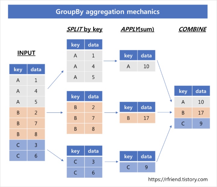
- pandas의 groupby() 연산자를 사용하여 집단, 그룹별로 데이터를 집계 및 요약을 할 수 있다.
- dataframe을 지정한 그룹으로 나누고, 각 그룹별로 집계합수를 적용하고, 그룹별 집계 결과를 하나로 합치는 과정을 거친다.
- 데이터 url : https://drive.google.com/drive/folders/149jcCyJFKKG5MFaPNWnYYqM2EkzgRz2P?usp=sharing
abalone_src = base_src+'/abalone.data'
abalone_df = pd.read_csv(base_src+'/abalone.data',
             header=None,sep=',',
             names=['sex','length','diameter','height',
                  'whole_weight','shucked_weight','viscera_weight',
                  'shell_weight','rings'])
abalone_df.head()
	sex   length diameter height whole_weight shucked_weight viscera_weight	shell_weight	rings
0	M	0.455	0.365	0.095	0.5140	0.2245	0.1010	0.150	15
1	M	0.350	0.265	0.090	0.2255	0.0995	0.0485	0.070	7
2	F	0.530	0.420	0.135	0.6770	0.2565	0.1415	0.210	9
3	M	0.440	0.365	0.125	0.5160	0.2155	0.1140	0.155	10
4	I	0.330	0.255	0.080	0.2050	0.0895	0.0395	0.055	7

# 데이터 shape 확인 => 4177개의 데이터와 9개의 변수
abalone_df.shape
> (4177, 9)

# 데이터 결측값 확인
abalone_df.isnull().sum().sum()
> 0

# 기술통계 확인(평균, 편차, 최소값, 25%, 50%, 75%, 최대값)
> 	length		diameter	height		whole_weight	shucked_weight	viscera_weight	shell_weight	rings
count	4177.000000	4177.000000	4177.000000	4177.000000	4177.000000	4177.000000	4177.000000	4177.000000
mean	0.523992	0.407881	0.139516	0.828742	0.359367	0.180594	0.238831	9.933684
std	0.120093	0.099240	0.041827	0.490389	0.221963	0.109614	0.139203	3.224169
min	0.075000	0.055000	0.000000	0.002000	0.001000	0.000500	0.001500	1.000000
25 %	0.450000	0.350000	0.115000	0.441500	0.186000	0.093500	0.130000	8.000000
50 %	0.545000	0.425000	0.140000	0.799500	0.336000	0.171000	0.234000	9.000000
75 %	0.615000	0.480000	0.165000	1.153000	0.502000	0.253000	0.329000	11.000000
max	0.815000	0.650000	1.130000	2.825500	1.488000	0.760000	1.005000	29.000000

# 전복 성별(M,F,I)에 따라 groupby함수를 통해 집계를 하겠다.
## 그룹별 합계 : grouped.sum()
## 그룹별 평균 : grouped.mean()
## 그룹별 크기 : grouped.size()
### ex) DataFrame[집계 변수].groupby(DataFrame[집계 대상])
grouped = abalone_df['whole_weight'].groupby(abalone_df['sex'])

# grouped는 pandas의 SeriesGroupBy object 형태이다.
grouped
> <pandas.core.groupby.generic.SeriesGroupBy object at 0x7f74f51f3f50>

grouped.sum()
>sex
  F    1367.8175
  I     578.8885
  M    1514.9500
Name: whole_weight, dtype: float64

grouped.mean()
>sex
  F    1.046532
  I    0.431363
  M    0.991459
Name: whole_weight, dtype: float64

grouped.size()
>sex
  F    1307
  I    1342
  M    1528
Name: whole_weight, dtype: int64

# 그룹변수 하나가 아닌, 전체 연속형 변수에 대한 집계
abalone_df.groupby(abalone_df['sex']).mean()
>	length		diameter	height	    whole_weight    shucked_weight	viscera_weight	shell_weight	rings
sex
F	0.579093	0.454732	0.158011	1.046532	0.446188	0.230689	0.302010	11.129304
I	0.427746	0.326494	0.107996	0.431363	0.191035	0.092010	0.128182	7.890462
M	0.561391	0.439287	0.151381	0.991459	0.432946	0.215545	0.281969	10.705497

# 다음과 같이 간단하게 작성할 수 있으며, 위와 같은 결과를 얻을 수 있다.
abalone_df.groupby('sex').mean()

# 새로운 조건에 맞는 변수 추가
abalone_df['length_bool'] = np.where(abalone_df['length']>abalone_df['length'].median(),
  				'length_long', # True일 경우
  				'length_short' # False일 경우)
abalone_df['length_bool']
>0       length_short
 1       length_short
 2       length_short
 3       length_short
 4       length_short
            ...
4172     length_long
4173     length_long
4174     length_long
4175     length_long
4176     length_long
Name: length, Length: 4177, dtype: object

# 그룹변수를 2개 이상 선택하여 총계처리
abalone_df.groupby(['sex','length_bool']).mean()
>                	 length		diameter	height	whole_weight	shucked_weight	viscera_weight	shell_weight	rings
 sex	length_bool
  F	length_long	0.626895	0.493020	0.169944	1.261330	0.542957	0.276945	0.360013	11.415073
 	length_short	0.477428	0.373301	0.132632	0.589702	0.240380	0.132311	0.178650	10.521531
  I	length_long	0.584495	0.452952	0.150957	0.923215	0.402524	0.196912	0.273247	10.585106
 	length_short	0.402210	0.305893	0.100997	0.351234	0.156581	0.074920	0.104549	7.451473
  M	length_long	0.623359	0.489291	0.168670	1.255182	0.554312	0.272203	0.351683	11.299172
	length_short	0.454875	0.353336	0.121664	0.538157	0.224335	0.118156	0.162141	9.685053

# 더 간결하게 표현한다면.
## 그룹변수('sex','length_bool') 선택 및 집계변수('whole_weight') 평균
abalone_df.groupby(['sex','length_bool'])['whole_weight'].mean()
>sex  length_bool
 F    length_long     1.261330
      length_short    0.589702
 I    length_long     0.923215
      length_short    0.351234
 M    length_long     1.255182
      length_short    0.538157
Name: whole_weight, dtype: float64

#> _'''위 글은 https://rfriend.tistory.com/383의 글을 참고하여 작성되었습니다.'''_
- 중복 데이터 삭제
# 기존 abalone 데이터 활용
abalone_df = pd.read_csv(base_src+'/abalone.data',
             header=None,sep=',',
             names=['sex','length','diameter','height',
                  'whole_weight','shucked_weight','viscera_weight',
                  'shell_weight','rings'])

# 중복된 row를 확인하는 법
abalaone_df.duplicated()
>0       False
1       False
2       False
3       False
4       False
        ...
4172    False
4173    False
4174    False
4175    False
4176    False
Length: 4177, dtype: bool

# 위와같이 하면 중복된 row를 확인할 수 있지만,
# 가시적으로 몇개가 중복되어 있는지 확인하기 어렵다.
abalone_df.duplicated().sum()
> 0

# 중복 예제 생성을 위해서, 가상으로 중복데이터 생성
## pd.concat은 2개의 DataFrame을 합치는 함수이다.
new_abalone_df = pd.concat([abalone_df,abalone_df.iloc[[0]]],axis=0)
new_abalone_df.duplicated()
>0       False
1       False
2       False
3       False
4       False
        ...
4173    False
4174    False
4175    False
4176    False
0        True
Length: 4178, dtype: bool

# keep='last' 옵션을 통해서 처음으로 중복되는 데이터를 검색
new_abalone_df.duplicated(keep='last')
>0       True
1       False
2       False
3       False
4       False
        ...
4173    False
4174    False
4175    False
4176    False
0        False
Length: 4178, dtype: bool

# 중복 데이터(row) 삭제
new_abalone_df.drop_duplicates()

# 중복 데이터(row) 삭제(첫번째 중복되는 것)
new_abalone_df.drop_duplicates(keep='last')

# 중복 데이터(column) 조회
new_abalone_df.duplicated('sex')

# 중복 데이터(column) 삭제
new_abalone_df.drop_duplicates('sex')

# 중복 데이터(column) 삭제(첫번째 중복되는 것)
new_abalone_df.drop_duplicates('sex')
- NaN(결측치) 찾아서 다른 값 변경
# 기존 avalone 데이터는 결측치가 존재하지 않는다.
abalone_df.isnull().sum().sum()
> 0

# 가상으로 결측치 생성
nan_abalone_df = abalone_df.copy()
nan_abalone_df.loc[2,'length'] = np.nan
>	sex	length	diameter	height	whole_weight	shucked_weight	viscera_weight	shell_weight	rings	length_bool
0	M	0.455	0.365	0.095	0.5140	0.2245	0.1010	0.1500	15	length_short
1	M	0.350	0.265	0.090	0.2255	0.0995	0.0485	0.0700	7	length_short
2	F	 NaN	0.420	0.135	0.6770	0.2565	0.1415	0.2100	9	length_short
3	M	0.440	0.365	0.125	0.5160	0.2155	0.1140	0.1550	10	length_short
4	I	0.330	0.255	0.080	0.2050	0.0895	0.0395	0.0550	7	length_short
...	...	...	...	...	...	...	...	...	...	...
4172	F	0.565	0.450	0.165	0.8870	0.3700	0.2390	0.2490	11	length_long
4173	M	0.590	0.440	0.135	0.9660	0.4390	0.2145	0.2605	10	length_long
4174	M	0.600	0.475	0.205	1.1760	0.5255	0.2875	0.3080	9	length_long
4175	F	0.625	0.485	0.150	1.0945	0.5310	0.2610	0.2960	10	length_long
4176	M	0.710	0.555	0.195	1.9485	0.9455	0.3765	0.4950	12	length_long

# 결측치를 특정 값으로 채우기
zero_abalone_df = nan_abalone_df.fillna(0)
zero_abalone_df
>	sex	length	diameter	height	whole_weight	shucked_weight	viscera_weight	shell_weight	rings	length_bool
0	M	0.455	0.365	0.095	0.5140	0.2245	0.1010	0.1500	15	length_short
1	M	0.350	0.265	0.090	0.2255	0.0995	0.0485	0.0700	7	length_short
2	F      "0.000"	0.420	0.135	0.6770	0.2565	0.1415	0.2100	9	length_short
3	M	0.440	0.365	0.125	0.5160	0.2155	0.1140	0.1550	10	length_short
4	I	0.330	0.255	0.080	0.2050	0.0895	0.0395	0.0550	7	length_short
...	...	...	...	...	...	...	...	...	...	...
4172	F	0.565	0.450	0.165	0.8870	0.3700	0.2390	0.2490	11	length_long
4173	M	0.590	0.440	0.135	0.9660	0.4390	0.2145	0.2605	10	length_long
4174	M	0.600	0.475	0.205	1.1760	0.5255	0.2875	0.3080	9	length_long
4175	F	0.625	0.485	0.150	1.0945	0.5310	0.2610	0.2960	10	length_long
4176	M	0.710	0.555	0.195	1.9485	0.9455	0.3765	0.4950	12	length_long

# 결측치를 결측치가 속한 컬럼의 평균값으로 대체하기
nan_abalone_df.mean()
>length          "0.523991"
diameter          0.407881
height            0.139516
whole_weight      0.828742
shucked_weight    0.359367
viscera_weight    0.180594
shell_weight      0.238831
rings             9.933684
dtype: float64

nan_abalone_df.fillna(nan_abalone_df.mean())
>	sex	length	diameter	height	whole_weight	shucked_weight	viscera_weight	shell_weight	rings	length_bool
0	M	0.455000	0.365	0.095	0.5140	0.2245	0.1010	0.1500	15	length_short
1	M	0.350000	0.265	0.090	0.2255	0.0995	0.0485	0.0700	7	length_short
2	F      "0.523991"	0.420	0.135	0.6770	0.2565	0.1415	0.2100	9	length_short
3	M	0.440000	0.365	0.125	0.5160	0.2155	0.1140	0.1550	10	length_short
4	I	0.330000	0.255	0.080	0.2050	0.0895	0.0395	0.0550	7	length_short
...	...	...	...	...	...	...	...	...	...	...
4172	F	0.565000	0.450	0.165	0.8870	0.3700	0.2390	0.2490	11	length_long
4173	M	0.590000	0.440	0.135	0.9660	0.4390	0.2145	0.2605	10	length_long
4174	M	0.600000	0.475	0.205	1.1760	0.5255	0.2875	0.3080	9	length_long
4175	F	0.625000	0.485	0.150	1.0945	0.5310	0.2610	0.2960	10	length_long
4176	M	0.710000	0.555	0.195	1.9485	0.9455	0.3765	0.4950	12	length_long
- apply 함수 활용
- DataFrame타입의 객체에서 호출가능한 apply함수에 대해 살펴보자.
- 본인이 원하는 행과 열에 연산 혹은 function을 적용할 수 있다.
- 열 기준으로 집계하고 싶은 경우 axis=0
- 행 기준으로 집계하고 싶은 경우 axis=1
abalone_df[['diameter']].apply(np.average,axis=0)
>diameter    0.407881
dtype: float64

# 열 기준 집계
abalone_df[['diameter','whole_weight']].apply(np.average,axis=0)
>diameter        0.407881
whole_weight    0.828742
dtype: float64

# 행 기준 집계
abalone_df[['diameter','whole_weight']].apply(np.average,axis=1)
>0       0.43950
1       0.24525
2       0.54850
3       0.44050
4       0.23000
         ...
4172    0.66850
4173    0.70300
4174    0.82550
4175    0.78975
4176    1.25175
Length: 4177, dtype: float64

# 사용자 함수를 통한 집계 ★★★★★
import math
def avg_ceil(x,y,z):
  return math.ceil((x+y+z)/3)

abalone_df[['diameter','height','whole_weight']].apply(lambda x : avg_ceil(x[0],x[1],x[2]),axis=1)
>0       1
1       1
2       1
3       1
4       1
       ..
4172    1
4173    1
4174    1
4175    1
4176    1
Length: 4177, dtype: int64

# 문제
  1. 사용자 정의 함수 사용
  2. ['diameter','height','whole_weight'] 변수 사용
  3. 세 변수의 합이 1이 넘으면 True, 아니면 False 출력 후 answer변수에 저장
  4. abalone_df에 answer 열을 추가하고 입력
- 컬럼 내 유니크한 값 뽑아서 갯수 확인
# 성별 변수에 포함된 M , I, F가 몇개인지 확인
abalone_df['sex'].value_counts()
>M    1528
I    1342
F    1307
Name: sex, dtype: int64

# 성별 변수에 포함된 M , I, F가 몇개인지 확인 및 정렬
abalone_df['sex'].value_counts(ascending=True)
>F    1307
I    1342
M    1528
Name: sex, dtype: int64

# 결측값이 있는 경우
abalone_df['sex'].value_counts(dropna=True)
- 두 개의 DataFrame 합치기
# 가상 abalone 1개 row데이터 생성 및 결합
one_abalone_df = abalone_df.iloc[[0]]
pd.concat([abalone_df,one_abalone_df],axis=0)
>	sex	length	diameter height	whole_weight	shucked_weight	viscera_weight	shell_weight	rings	length_bool
0	M	0.455	0.365	0.095	0.5140	0.2245	0.1010	0.1500	15	length_short
1	M	0.350	0.265	0.090	0.2255	0.0995	0.0485	0.0700	7	length_short
2	F	0.530	0.420	0.135	0.6770	0.2565	0.1415	0.2100	9	length_short
3	M	0.440	0.365	0.125	0.5160	0.2155	0.1140	0.1550	10	length_short
4	I	0.330	0.255	0.080	0.2050	0.0895	0.0395	0.0550	7	length_short
...	...	...	...	...	...	...	...	...	...	...
4173	M	0.590	0.440	0.135	0.9660	0.4390	0.2145	0.2605	10	length_long
4174	M	0.600	0.475	0.205	1.1760	0.5255	0.2875	0.3080	9	length_long
4175	F	0.625	0.485	0.150	1.0945	0.5310	0.2610	0.2960	10	length_long
4176	M	0.710	0.555	0.195	1.9485	0.9455	0.3765	0.4950	12	length_long
0	M	0.455	0.365	0.095	0.5140	0.2245	0.1010	0.1500	15	length_short

# 가상 abalone 1개 col 데이터 생성 및 결합
one_abalone_df = abalone_df.iloc[:,[0]]
pd.concat([abalone_df,one_abalone_df],axis=1)
>sex	length	diameter height	whole_weight	shucked_weight	viscera_weight	shell_weight	rings	length_bool	sex
0	M	0.455	0.365	0.095	0.5140	0.2245	0.1010	0.1500	15	length_short	M
1	M	0.350	0.265	0.090	0.2255	0.0995	0.0485	0.0700	7	length_short	M
2	F	0.530	0.420	0.135	0.6770	0.2565	0.1415	0.2100	9	length_short	F
3	M	0.440	0.365	0.125	0.5160	0.2155	0.1140	0.1550	10	length_short	M
4	I	0.330	0.255	0.080	0.2050	0.0895	0.0395	0.0550	7	length_short	I
...	...	...	...	...	...	...	...	...	...	...	...
4172	F	0.565	0.450	0.165	0.8870	0.3700	0.2390	0.2490	11	length_long	F
4173	M	0.590	0.440	0.135	0.9660	0.4390	0.2145	0.2605	10	length_long	M
4174	M	0.600	0.475	0.205	1.1760	0.5255	0.2875	0.3080	9	length_long	M
4175	F	0.625	0.485	0.150	1.0945	0.5310	0.2610	0.2960	10	length_long	F
4176	M	0.710	0.555	0.195	1.9485	0.9455	0.3765	0.4950	12	length_long	M
결론
오늘부로 데이터전처리의 기본 실습이 끝났다. 오늘 배운 것들이 가령 어디에 쓰일지 지금 이해를 못해도 괜찮다. 만약 이 글을 읽은 여러분들이 데이터 전처리를 할 시점이 되었을 때, 오늘 읽었던 내용이 머리에 조금이나마 스쳐지나간다면 오늘의 노력은 정말 의미있고 가치있어 질 것이다.

데이터 분석 유튜버 "거친코딩"입니다.
안녕하세요. 영상 꾸준히 잘보고있습니다.
다름이 아니라 궁금한 점이 있어서 글을 남깁니다.
데이터 결측값 확인할 때 abalone_df.isnull().sum().sum() 을하면 0이 나오던데
저는 4180이 나와서요 이런건 왜그런것인지 왜 다른 것인지가 좀 궁금합니다...!