[Section8] Pandas with Date/Time

해당 내용은 Udemy 강의 'Pandas 및 Python을 이용한 데이터 분석:마스터 클래스'를 수강 후 정리한 내용입니다.

https://www.udemy.com/course/best-pandas-python

Section1

BASIC PYTHON DATETIME MODULE

# datetime is one of Python's core standard libraries
# We are going to use two methods to deal with dates/times: (1) date and (2) dateime
# date: helps us define dates only without including time (month, day, year)
# datetime: helps us define times and dates together (month, day, year, hour, second, microsecond)

import pandas as pd
import datetime as dt
import calendar 

# Pick a date using Python's date method inside the datetime module
my_date = dt.date(2020, 3, 22)
my_date

# Convert it into string to view the date and time
str(my_date)

my_date.day, my_date.month,my_date.year와 같은 attribute 사용 가능

# Let's define a datetime using datetime method as follows
my_datetime = dt.datetime(2020, 3, 22, 8, 20, 50)

my_datetime.hour, my_date.minute,my_date.second와 같은 attribute 사용 가능

# print out calendar!
import calendar 
print(calendar.month(2021, 3))

# You can also use pd.datetime to convert a regular Pandas Series into datetime as follows:

dates = pd.Series(['2020/03/20', '2020-08-25', 'March 22nd, 2020'])
dates

# The to_datetime() method converts the date and time in string format to a DateTime object:
my_dates = pd.to_datetime(dates, format='mixed')
my_dates

MINI CHALLENGE #1:

• Use Python's datetime method to write your date and time of your birth! Convert it into string format

my_birthday = dt.datetime(1999, 7, 11, 12, 5)

str(my_birthday)

---

Section2

HANDLING DATES AND TIMES USING PANDAS

# Timestamp is the pandas equivalent of python’s Datetime and is interchangeable with it in most cases.
# It’s the type used for the entries that make up a DatetimeIndex, and other timeseries oriented data structures in pandas.

pandas.Timestamp — pandas 2.2.3 documentation

pd.Timestamp('2020, 3, 22, 10')

# Or you can define a Pandas Timestamp using Python datetime object

pd.Timestamp(dt.datetime(2020, 3, 22 ,8, 20, 50))

# Calculate difference between two dates
day_1 = pd.Timestamp('1998, 3, 22, 10')
day_2 = pd.Timestamp('2021, 3, 22, 10')
delta = day_2-day_1
print(delta)

# Let's define 3 dates for 3 separate transactions

date_1 = dt.date(2020, 3, 22)
date_2 = dt.date(2020, 4, 22)
date_3 = dt.date(2020, 5, 22)

# Let's put the 3 dates in a list as follows

dates_list = [date_1, date_2, date_3]

# Use Pandas DateTimeIndex to convert the list into datetime datatype as follows
# Datetime index constructor method creates a collection of dates

dates_index = pd.DatetimeIndex(dates_list)

# Define a list that carries 3 values corresponding to store sales

sales = [50, 55, 60]

# Define a Pandas Series using datetime and values as follows:

sales = pd.Series(data=sales, index=dates_index)
print(sales)

# you can also define a range of dates as follows:

my_days = pd.date_range(start='2020-01-01', end='2020-04-01', freq='D')
my_days

# you can also define a range of dates using M which stands for month end as follows:
# last day of month

my_days = pd.date_range(start='2020-01-01', end='2020-08-01', freq='M')
my_days

# Alternative way of defining a list of dates

pd.date_range(start='2020-01-01', periods=20, freq='D')

freq Parameter

날짜 관련

옵션	의미	예시 (start="2024-01-01", periods=5)
D	일 단위 (주말 포함)	2024-01-01, 2024-01-02, 2024-01-03, 2024-01-04, 2024-01-05
B	평일(월~금) 단위	2024-01-01, 2024-01-02, 2024-01-03, 2024-01-04, 2024-01-05
W	주 단위 (일요일 기준)	2024-01-07, 2024-01-14, 2024-01-21, 2024-01-28, 2024-02-04
W-MON	주 단위 (월요일 기준)	2024-01-01, 2024-01-08, 2024-01-15, 2024-01-22, 2024-01-29

시간 관련

옵션	의미	예시 (start="2024-01-01", periods=5)
H	시간 단위	2024-01-01 00:00, 01:00, 02:00, 03:00, 04:00
T or min	분 단위	2024-01-01 00:00, 00:01, 00:02, 00:03, 00:04
S	초 단위	2024-01-01 00:00:00, 00:00:01, 00:00:02, 00:00:03, 00:00:04

월/분기/연도 관련

옵션	의미	예시 (start="2024-01-01", periods=5)
M	월 마지막 날	2024-01-31, 2024-02-29, 2024-03-31, 2024-04-30, 2024-05-31
MS	월 첫째 날	2024-01-01, 2024-02-01, 2024-03-01, 2024-04-01, 2024-05-01
Q	분기 마지막 날	2024-03-31, 2024-06-30, 2024-09-30, 2024-12-31
Q-JAN	1월 시작 분기 마지막 날	2024-04-30, 2024-07-31, 2024-10-31, 2025-01-31
Y	연도 마지막 날	2024-12-31, 2025-12-31, 2026-12-31, 2027-12-31, 2028-12-31
YS	연도 첫째 날	2024-01-01, 2025-01-01, 2026-01-01, 2027-01-01, 2028-01-01

숫자를 붙히면 주기를 조절할 수 있다.

pd.date_range(start="2024-01-01", periods=5, freq="2D")  # 이틀 간격
pd.date_range(start="2024-01-01", periods=5, freq="3B")  # 평일 3일 간격
pd.date_range(start="2024-01-01", periods=5, freq="4H")  # 4시간 간격

MINI CHALLENGE #2:

• Obtain the business days between 2020-01-01 and 2020-04-01

# 2020-01-01부터 2020-04-01까지의 평일(월~금) 날짜 생성
weekdays = pd.date_range(start="2020-01-01", end="2020-04-01", freq='B')

print(weekdays)

---

Section3

DATETIME IN ACTION! PRACTICAL EXAMPLE PART #1

# dataframes creation for both training and testing datasets

avocado_df = pd.read_csv('avocado.csv')

# Convert date column to datetime format
avocado_df['Date'] = pd.to_datetime(avocado_df['Date'])
avocado_df

# Date: The date of the observation
# AveragePrice: the average price of a single avocado
# type: conventional or organic
# Region: the city or region of the observation
# Total Volume: Total number of avocados sold

# You can select any column to be the index for the DataFrame

avocado_df.set_index(keys=['Date'], inplace=True)

avocado_df.values

avocado_df.columns

avocado_df.index

MINI CHALLENGE #3:

• What are the datatypes of each column in the avocado_df DataFrame?

avocado_df.info()

---

Section4

DATETIME IN ACTION! PRACTICAL EXAMPLE PART #2

# access elements with a specific datetime index using .loc

avocado_df.loc['2018-01-21']

# You can use iloc if you decide to use numeric indexes

avocado_df.iloc[5]

# Truncate a sorted DataFrame given index bounds.
# Make sure to sort the dataframe before applying truncate
# 18249 rows -> 6154 rows

avocado_df = avocado_df.sort_index()  # 인덱스 정렬

avocado_df = avocado_df.truncate('2017-01-01', '2018-02-01')
avocado_df 

# Access more than one element within a given date range
# 인덱스가 정렬되지 않은 상태에서 특정 날짜 범위를 조회하면 오류 발생 

avocado_df.loc['2017-01-04':'2018-01-25'] 

# you can offset (shift) all dates by days or month as follows

avocado_df.index = avocado_df.index + pd.DateOffset(months=12, days=30)

# Let's revert back to the original dataset!

avocado_df.index = avocado_df.index - pd.DateOffset(months=12, days=30)
avocado_df

# Once you have the index set to DateTime, this unlocks its power by performing aggregation
# Aggregating the data by year (A = annual)

# 숫자형 데이터만 선택하여 평균 계산
# avocado_df.select_dtypes(include='number').resample('A').mean()

avocado_df.select_dtypes(include='number').resample('YE').mean()

: 'A' is deprecated and will be removed in a future version, please use 'YE' instead.

# Aggregating the data by month (M = Month)

# avocado_df.select_dtypes(include='number').resample(rule ='M').mean()

avocado_df.select_dtypes(include='number').resample(rule ='ME').mean()

: 'M' is deprecated and will be removed in a future version, please use 'ME' instead.

# You can obtain the maximum value for each Quarter end as follows:

# avocado_df.select_dtypes(include='number').resample(rule ='Q').max()
avocado_df.select_dtypes(include='number').resample(rule ='QE').max()

: 'Q' is deprecated and will be removed in a future version, please use 'QE' instead.

# You can locate the rows that satisfies a given critirea as follows:

low_price = avocado_df['AveragePrice'].where(avocado_df['AveragePrice']<1.2)
low_price

# 기준을 만족하는 월별 AveragePrice의 개수

low_price = avocado_df['AveragePrice'].where(avocado_df['AveragePrice']<1.3).resample('1ME').count()
low_price

# Date column에서 일(Day)에 해당하는 정보 추출하여 새로운 칼럼 생성

avocado_df['Day'] = avocado_df['Date'].dt.day

# Date column에서 월(Month)에 해당하는 정보 추출하여 새로운 칼럼 생성

avocado_df['Month'] = avocado_df['Date'].dt.month

# Date column에서 연(Year)에 해당하는 정보 추출하여 새로운 칼럼 생성

avocado_df['Year'] = avocado_df['Date'].dt.year
avocado_df

MINI CHALLENGE #4:

• Calculate the average avocado price per quarter end

avocado_df.select_dtypes(include='number').resample(rule ='QE').mean()

---

Section5

DATA PLOTTING (STRETCH ASSIGNMENT!)

# Once you have index set to DateTime, this unlocks its power by performing aggregation
# Aggregating the data by month end

avocado_df.select_dtypes(include='number').resample(rule ='ME').mean()

# plot the avocado average price per month

avocado_df.select_dtypes(include='number').resample(rule ='ME').mean()['AveragePrice'].plot(figsize=(10,5), marker='o', color='r')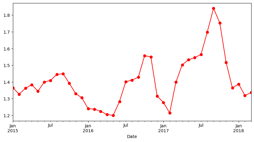

# plot the avocado average price per quarter

avocado_df.select_dtypes(include='number').resample(rule ='QE').mean()['AveragePrice'].plot(figsize=(10,5), marker='o', color='r')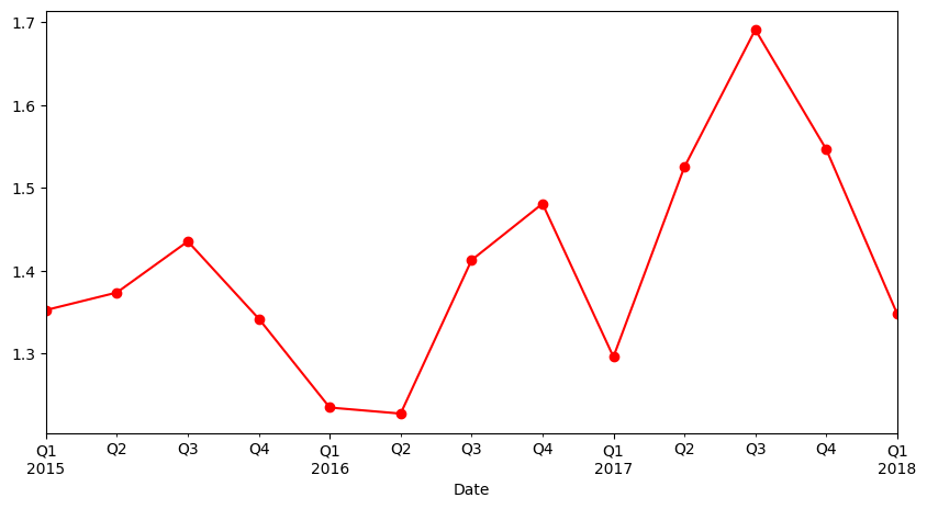

# plot the avocado average price per annual basis

avocado_df.select_dtypes(include='number').resample(rule ='YE').mean()['AveragePrice'].plot(figsize=(10,5), marker='o', color='r')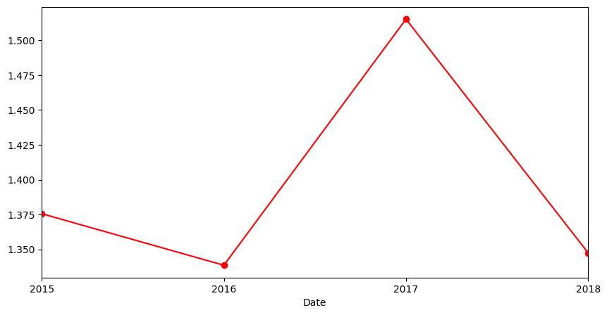

import seaborn as sns
import matplotlib.pyplot as plt

plt.figure(figsize = (10, 7))
sns.violinplot(y = 'AveragePrice', x = 'type', data = avocado_df, palette='Set1')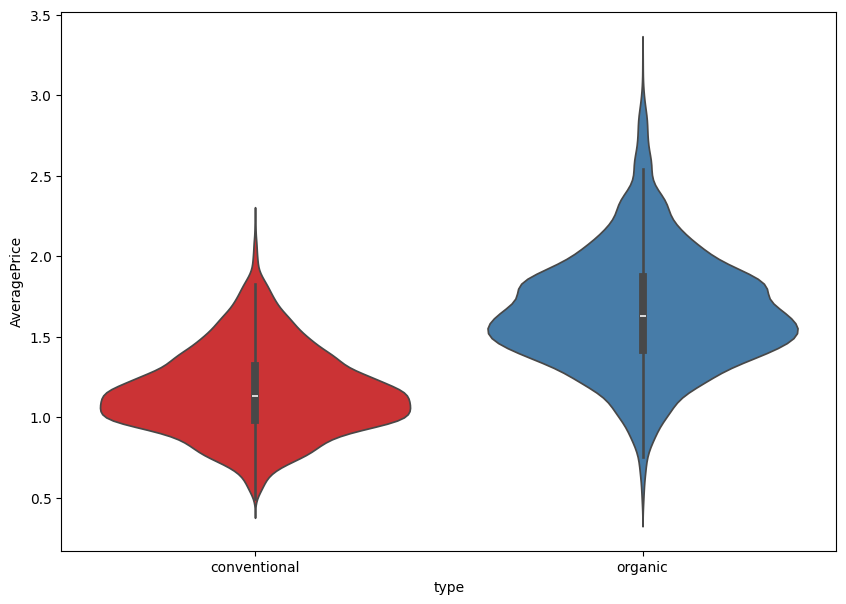

# plot the distribution plot of avocado prices (histogram + Kernel Denisty Estimate)

plt.figure(figsize=(13,6))
sns.distplot(avocado_df['AveragePrice'], color='b')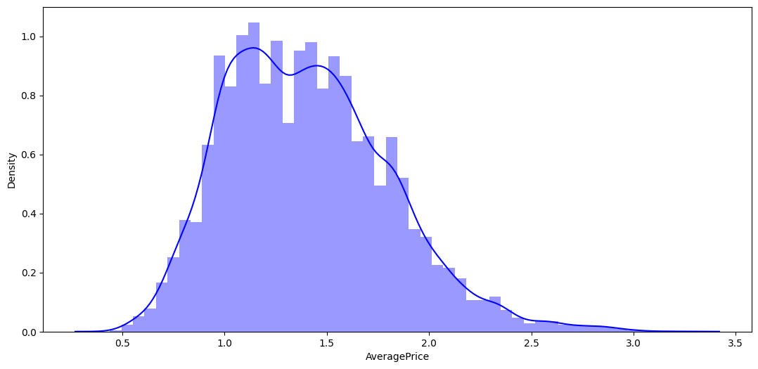

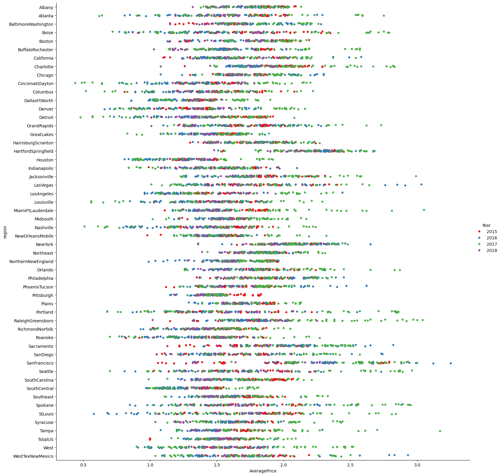
# Catplot is used to draw categorical plots onto a FacetGrid.
# Catplot provides access to several axes-level functions that show the relationship between a numerical and one or more categorical variables.

conventional = sns.catplot(x='AveragePrice', y='region', data=avocado_df[avocado_df['type'] == 'conventional'], hue='Year', height=10, palette='Set1')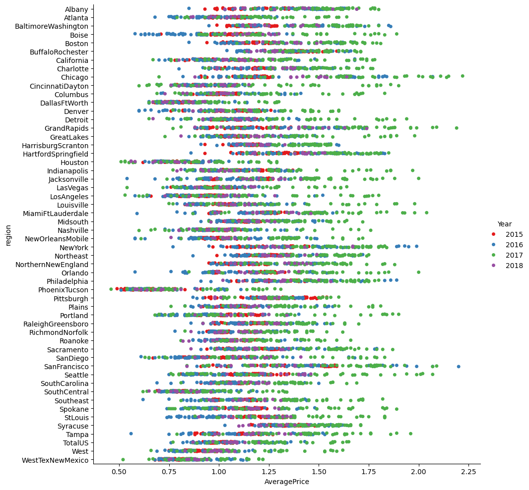

MINI CHALLENGE #5:

• Plot the average price of avocado on a weekly basis
• Plot Catplot for price vs. region for organic food

# Plot the average price of avocado on a weekly basis
avocado_df.select_dtypes(include='number').resample(rule ='W').mean()['AveragePrice'].plot(figsize=(10,5), marker='o', color='r')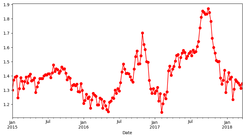

# Plot Catplot for price vs. region for organic food
organic = sns.catplot(x='AveragePrice', y='region', data=avocado_df[avocado_df['type'] == 'organic'], hue='Year', height=16, palette='Set1')

---