Lecture 08. Data Splits, Models & Cross-Validation

Lecture video link: https://youtu.be/rjbkWSTjHzM

Outline

• Bias / Variance $\sim$ easy to understand, but hard to master
• Regularization $\sim$ how to reduce variance in learning algorithms
• Train/dev/test splits
• Model selection vs. Cross validation

Bias & Variance

Bias

An error from erroeous assumptions in the learning algorithm.

Technically, $\text{bias}=|\text{average model prediction}-\text{ground truth}|$.

Characterisitics

• Failure to capture proper data trends
• Potential towards underfitting
• More generalized/overly simplified
• High error rate

Variance

An error from sensitivity to small fluctuations in the tarining set.

The changes in the model when using different portions of the training dataset.

Characteristics

• Noise in the dataset
• Potentials towards overfitting
• Complex models
• Trying to put all data points as close as possible

(Ref links:

https://en.wikipedia.org/wiki/Bias–variance_tradeoff,

https://www.bmc.com/blogs/bias-variance-machine-learning/)

Price vs. size of house (ex.)

$\theta_0+\theta_1x$

Underfit

High bias

$\theta_0+\theta_1x+\theta_2x^2$

Just right

$\theta_0+\theta_1x+\cdots+\theta_5x^5$

Overfit

High variance

One of the ways to prevent overfitting is regularization.

Regularization

Comment: it’ll sound deceptively simple but is one of the techniques that I use most often in many models.

ex. For linear regression,

Large $\lambda$ → underfitting.

$\lambda=0$ → relatively overfitting.

Q. Have you ever regularized multiple elements of parameters?

A. Not really. Choosing parameters $\lambda_i$’s corresponding to each $\theta_i$ is as difficult as just choosing all the parameters $\lambda_i$’s in the first place. When we cover cross-validation and multiple regression, we’ll learn how to choose $\lambda$, but the technique won’t work for choosing from multiple number of $\lambda_i$’s.

Logistic regression with regularization will usually outperform naive Bayes on a classification accuracy standpoint. Without regularization, logistic regression will badly overfit the given data. (e.g. $m=100$ e-mails to classify as spam or non-spam; $n=10000$ words.)

Q. Why don’t SVMs suffer too badly? Is it because there are a small number of vectors or is it because of minimizing the penalty $w$?

A. I would say the formal argument relies more on the latter, but actually both. The class of all functions that separate the data of a large margin is a relatively simple class of functions, which I mean has low VC dimension, and thus any function within that class of functions is unlikely to overfit.

Q. Are the terms underfitting and high bias, or the terms overfitting and high variance interchangeable?

A. Not really. You can imagine a decision boundary with high bias and high variance: a very complicated function which still doesn’t fit your data well for some reason.

$S=\{x^{(i)},y^{(i)}\}_{i=1}^m$: training set

Assume a prior distribution $p$ over $\theta$ exists. This allows us to treat $\theta$ as a random variable as in Bayesian statistics.

(ref: https://en.wikipedia.org/wiki/Maximum_a_posteriori_estimation)

Recall that

by Bayes rule. And MLE would become

where we assumed $\theta\sim\mathcal{N}(0,\tau^2I)$, or

cf. Statistics: Frequentist vs. Bayesian?

For frequentist,

(cf. $\theta$ is a paramter here.)

For Bayesian,

where MAP stands for maximum a posteriori. (cf. $\theta$ is treated as a random variable here.)

Q. Can differences between these two (MLE and MAP) be seen as “regularized” vs. “non-regularized”?

A. Yes. MLE corresponds to the origin of regularization and the latter procedure (Bayesian) corresponds to adding regularization.

(Further description of differences between frequentist and Bayesian:

https://www.redjournal.org/article/S0360-3016(21)03256-9/fulltext#seccesectitle0004)

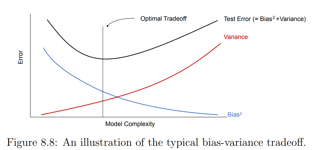
Error vs. Model complexity

Model complexity e.g. degree of polynomial

→ Higher the degree of your polynomial, the greater your training error.

e.g.

$\lambda=10^{100}$ → underfit

$\lambda=0$ → overfit

(Source: cs229-notes.pdf — Google it.)

Train/dev/test sets

$S\rightarrow S_{\text{train}}, S_{\text{dev}}, S_{\text{test}}$

• Train each model $i$ (option for degree of polynomial) on $S_{\text{train}}$. Get some hypothesis $h$.
• Measure error on $S_{\text{dev}}$. Pick model with the lowest error on $S_{\text{dev}}$. (Why not no $S_{\text{train}}$? To avoid overfit.)
  
• Optional: Evaluate algorithm on $S_{\text{test}}$ and report the error.

Comment: Reporting on the dev error isn’t really a valid unbiased procedure.

Split ratio?

→ train : test = 7 : 3; train : dev : test = 6 : 2 : 2 (great)

(Simple) Hold-out cross-validation

“development set” = “cross-validation set”

For small datasets…

ex. $m=100$

→ $70\;S_{\text{train}}, 30\;S_{\text{dev}}.$

$k$-fold CV(cross-validation)

$k=10$ is typical.

For $i=1,\cdots,k,$

Train (fit parameters) on $k-1$ pieces.

Test on reaming $1$ piece.

Average.

Optional: refit the model on all 100% of data.

Leave-on-out CV

$k=m$.

You need to change your algorithm $m$ times. → The huge downside… (very very expensive)

You never do this unless $m$ is too small. (e.g. $m\le100$ → you could consider this..)

Q. How do you sample the data in these sets?

A. In this lecture, we assume all your data comes from the same distribution, so we just randomly shuffle.

More to ref: mlyearning.org (machine learning yearning) or CS230. (if the train and test sets are from different distributions.)

Feature selection

Start with $\mathcal{F}=\phi.$

Repeat {

1. Try adding each feature $i$ to $\mathcal{F}$ and see which single-feature addition most improves the dev set performance.
2. Add that feature to $\mathcal{F}$.

}