Computer Vision in Game
For Immersion(몰입감)
• Eye Tracking for Enhanced Interaction
(강력한 상호작용을 위한 아이트래킹)
• Gesture Recognition for Intuitive Controls
(직관적인 컨트롤을 위한 제스쳐 인식)
• Facial Recognition for Personalized Gameplay
(개인에 특화된 플레이를 위한 안면 인식)
• Realizing Immersion through Visual Effects
(시각 효과를 통한 몰입감 실현)
• High-Quality Graphics and Realistic Environments
(고퀄리티 그래픽과 현실감 있는 환경)
• Dynamic Lighting and Shadow Effects
(움직이는 빛과 그림자 효과)
For Graphics
• Object Detection(물체 탐지)
• Instance Segmentation(분할)
• Text recognition(텍스트 인식)
• Object Tracking(물체 추적)
• 3D reconstruction(3D 건축)
• Image Generation(이미지 생성)
• Style Transfer(변환)
한계
• Hardware Limitations and Performance Optimization
(하드웨어 제한과 성능 최적화)
• Privacy and Ethical Considerations
(프라이버시와 윤리적 고려)
AI
Perceptron
Thresholding logic(임계 논리)
A McCulloch Pitts unit
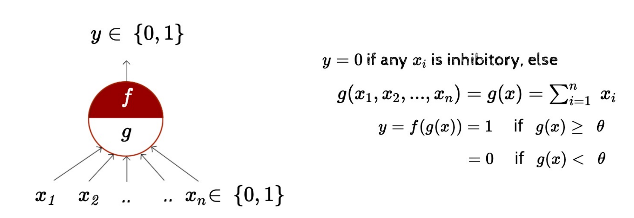
- 초기 퍼셉트론 모델
OR Function
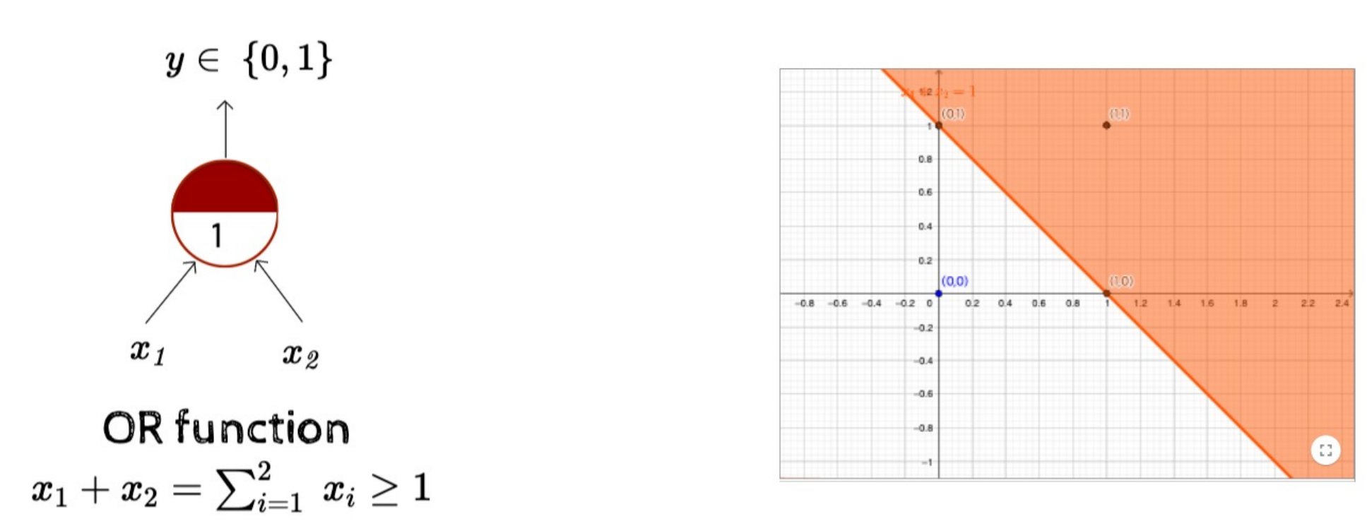
- Input이 하나라도 1이면 return 1
- 선형 분리
Classical perceptron model

- OR function에 input 값마다 가중치(weight)를 부여해서 계산함
- boolean function을 왜 구현해야 하나
- 왜 가치가 필요한가
- w0 = -θ 이 왜 편향이라 불리나
❗Error Control
💡 weight 값을 조정하며 최적의 결과와 최소한의 오류를 가지는 값을 찾아내는 것이 목표
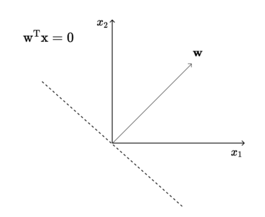
1로 나오는애들은 w와 각도가 90도 이하이고 0이 나오는애들은 w와 각도가 90도보다 크다는 것. 이게 만족할때까지 (수렴할때까지)계속 반복문 돌리면서 w 업데이트
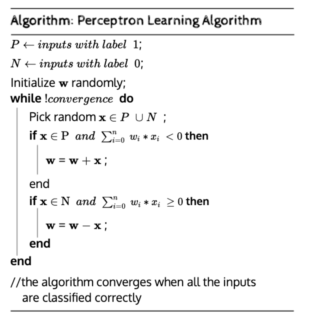
- 벡터의 내적으로 생각하면 됨
한계
- 싱글 퍼셉트론 방식은 non-linear 문제 해결이 어려움
해결방법
선형 분리(linearly separable) 가능하게 만들기
- 점의 개수 감소시키기
- 차원 증가시키기
- 멀티 레이어 적용
MLP
Multi-Layer Perceptron
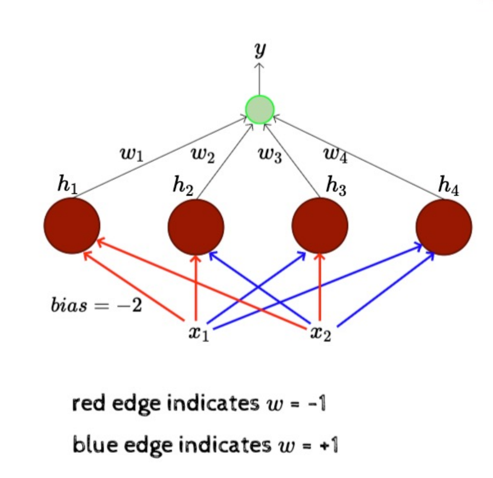
3 layers
input layer: x1, x2hidden layer: h1~h4 중간 계층 퍼셉트론output layer: 하나의 출력 뉴런(최종 계층)
- XOR 같은 문제도 해결 가능(비선형 문제 해결 가능)
- 3개 보다 더 많은 input이 있으면?
- 2^N 개의 퍼셉트론 필요
Multilayerd Perceptrons (MLP) 정리
• input, output, 하나 이상의 hideen layer 존재
• 하나의 hidden layer를 가진 MLP의 표현력
• 어떠한 boolean 함수도 구현 가능(어떠한 비선형 문제도 구현)
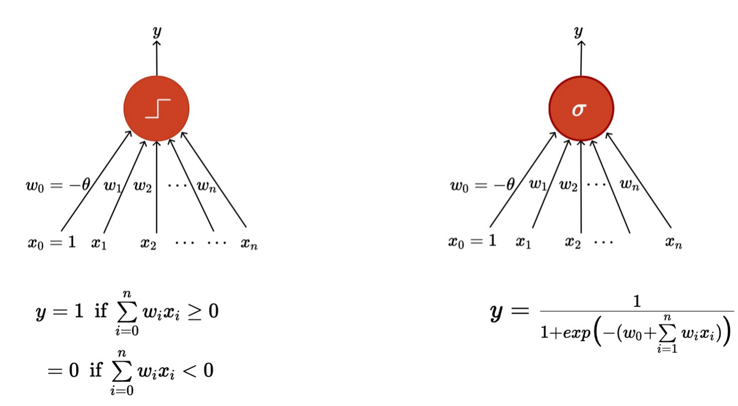
Sigmoid Neurons
Thresholding logic(임계 논리)
- thresholding logic을 이용하면 극단적으로 표현됨
- ex) 0.51 vs 0.49
- 계단 함수처럼 표현됨
- 실사용하려면 더 부드러운 표현이 필요!
Sigmoid Function
- 출력 함수가 thresholding logic에 비해 부드러움
- Binary가 아님(0~1 사이 값이긴 함)
- 결정적x, 확률적
Sigmoid Activition
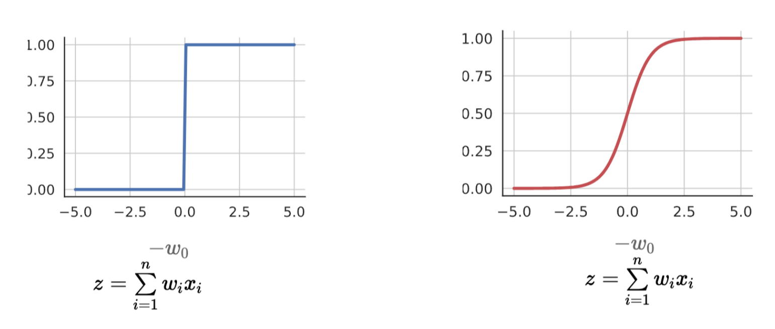
- sigmoid function 특징: 미분 가능, 연속적, 부드러움
Supervised Learning(지도 학습)
- weight를 어떻게 학습하나
- 에러 0은 힘들다 ➡️ 가능한 적은 에러 도달 목표
- 가중치를 학습 후 새로 입력되는 x로부터 출력값 d를 예측하기
Notation
- Data: { x^(n), D^(n) }
- Model: x와 d의 관계 근사
- w(가중치)를 입력<- 데이터로부터 학습 필요
- 적절한 모델과 알고리즘을 찾기 => 에러 최소화
- Algorithm: LMS, Logistic sigmoid (minimizing loss function)
- X를 입력 받았을 때, D를 출력하는 함수(모델)를 approximation 하는 것이 목표.
Error Surface
- (w, b)의 에러가 최소화 되는 점을 찾기
- 근데 파라미터가 늘어나면 찾기 어려움
=> Gradient를 쓰자!
Gradient
Gradient : 기울기가 가장 크게 증가하는 방향

LMS
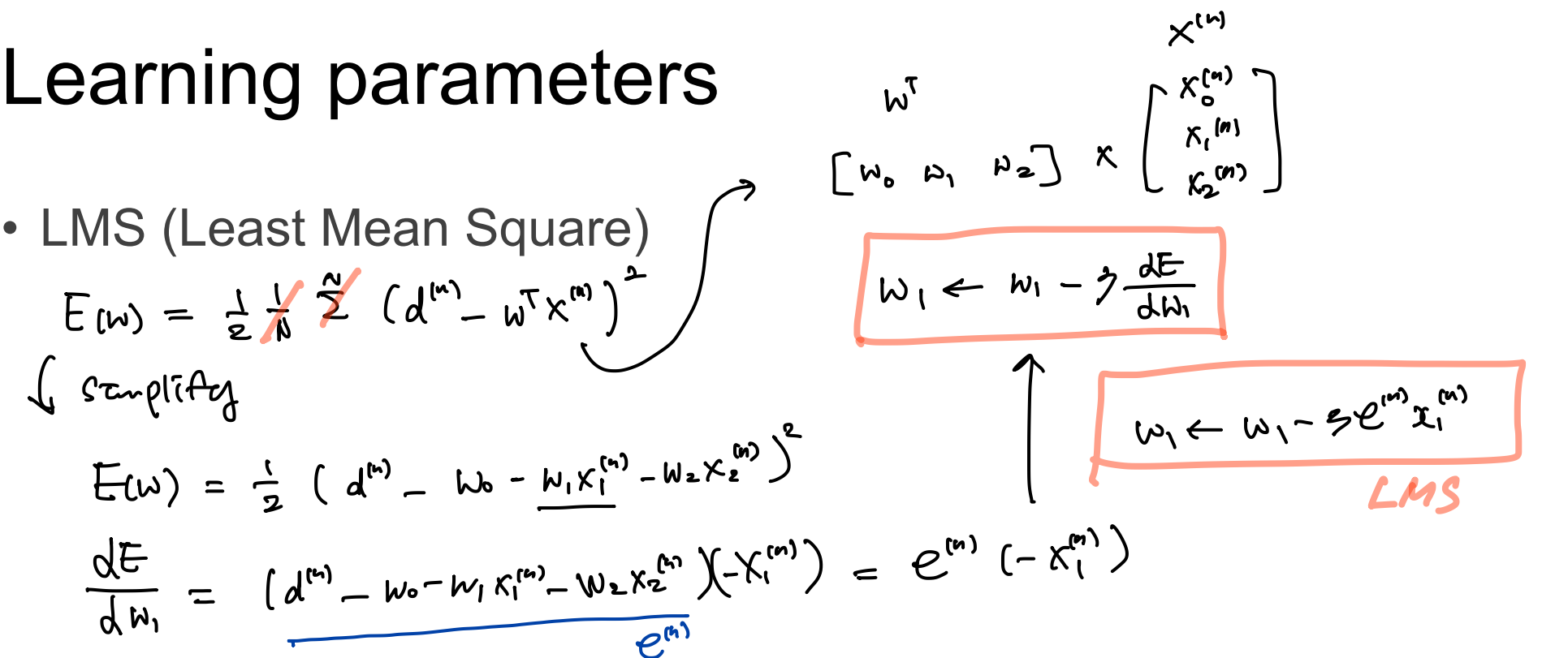
- 사실 식은 잘 모르겠지만 여튼 오차가 제일 작은 값을 찾아내는 방법!
Activation function
- 이것도 있음 ㅇㅇ
MLP Gradient Decent
Multi Layer Perceptrons
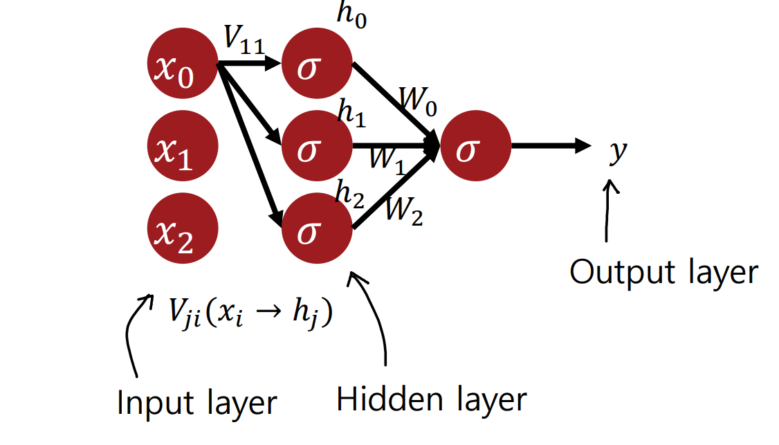
- y값을 내는 과정 → Hidden layer에 있는 각각의 Sigmoid Function에서 나온 결과 h와 W를 곱해서 한번더 Sigmoid Function을 거쳐 나온 것
Back Propagation
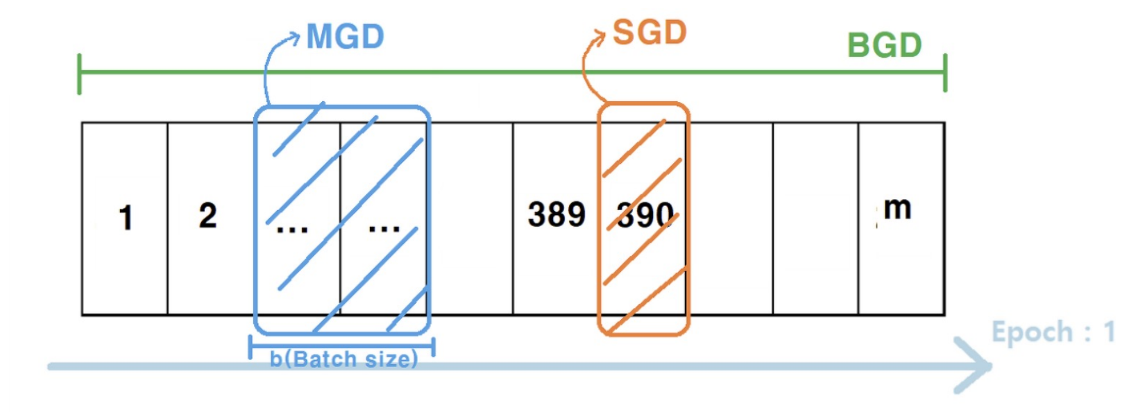
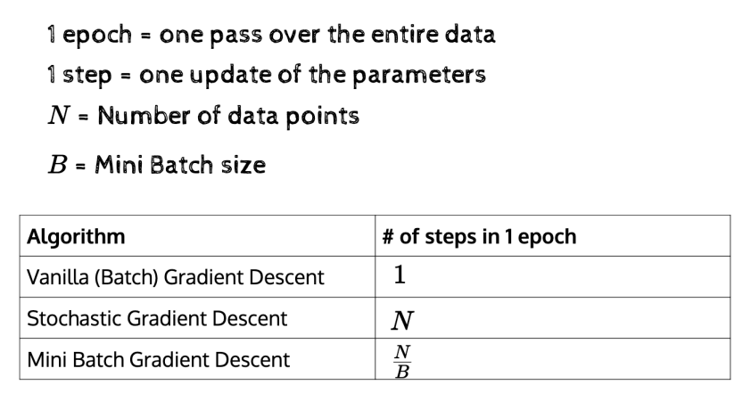
Stochastic Grandient Decent (SGD)
- 데이터 하나를 받은 후 forward pass를 실행하고, 에러를 계산하고, backpropagate를 에러에 대해 실행하고, weight값을 업데이트
Batch Gradient Decent (BGD)
- BGD는 모든 데이터 셋에 대하여 한 번에 계산을 진행하므로 메모리 사용률이 큼. 대신 정확함. 느리지만 정확하다.
BGD: 모든 데이터를 다 계산 후 에러 Gradient를 생성하여 평균값으로 업데이트를 진행하기에 오래걸리지만 신뢰도가 높고 안정적임.
- 메모리 사용률 큼, 정확함
SGD: BGD보다는 local하게 보는 방법이고, 빠르긴 하지만, 노이즈 데이터가 있을 경우 결과가 이상하게 나올 가능성이 있음. 굉장히 많은 단계를 거쳐 업데이트를 진행하기때문에 Iteration(얼마나 업데이트를 많이 하냐)이 데이터의 수 만큼 이뤄짐.- 빠르다, 많은 반복 필요
Mini-batch Gradient Decent (MGD)
총정리
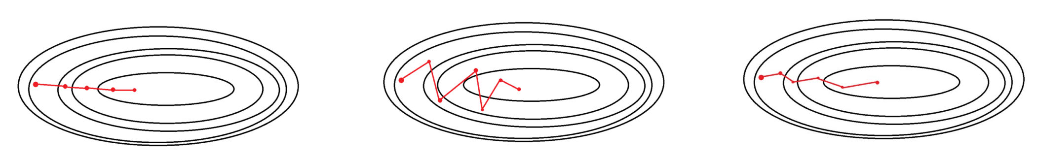
BGD
- 전체 데이터셋을 하나의 batch로 봄
- 업데이트가 최소
- 안정되게 수렴함
- 가장 많은 메모리를 요구(한번에 계산하니까)
SGD
- 전체 데이터셋 중 하나씩 계산 (batch size 1)
- 각각 적용해서 방향이 휙휙 바뀜
- 데이터가 작아서 빠르게 학습함
- 전체적으로 작게 수렴하는 것이 어려움
- 노이즈가 큼
MGD(절충안)
- 데이터를 일정 크기로 쪼개서 학습에 사용함
- 컴퓨팅 자원 적게 쓰고 빠름
Gradient Decent
BGD vs SGD vs MGD
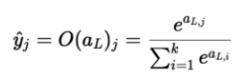
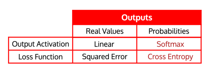
Softmax
- 해당 노드의 확률 값 / 모든 노드의 확률 값 으로 나타낸다. 정규화를 위한 함수
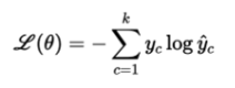
Loss function: Cross Entropy
- 머신 러닝 분류 모델의 발견된 확률 분포와 예측 분포 사이의 차이를 측정
- 결과 값이 3개 이상일 경우에 주로 사용(2개는 Binary Cross Entropy)
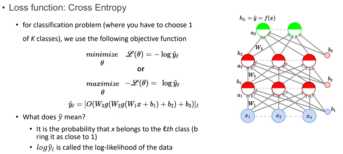
- y가 뜻하는 것
- x가 ℓ번째 클래스에 속할 확률(1에 가깝게 만든다)
- log y는 로그 확률(log-likelihood)라 부른다
- 정답이 되는 y값만이 1로 표현되고, 나머지 데이터들은 0으로 표현되는 one-hot vector의 형태이므로 결국 loss는 정답 데이터만을 포함한 수식으로 나타낼 수 있음
- model output과 true label의 cross entropy를 최소화하는 방향으로 동시에 likelihood를 최대화 하는 방향으로 학습을 진행한다.
- 결국 cross entropy를 최소화 하는게 log likelihood를 최대화하겠다는 것과 같은 말이다.
MSE와 CE 중에 뭐가 더 수렴이 잘 되나?
- CE loss가 더 빨리 수렴한다(분류 문제에서)
- soft plus function의 그래프 모양 (wrong일 비교적 더 큰 error값을)
- 연속적 분포 데이터(Regression) -> MSE
- 이산적 분포 데이터(Classification) -> CEE
Convergence speed
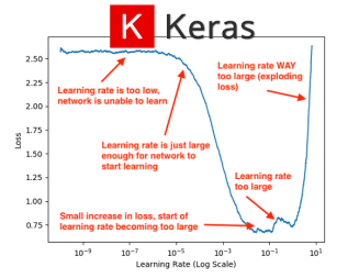
Learning rate
- learning rate 조절[다른 값으로 log scale을 조절한다. ex) 0.001, 0.01 등]
- 몇 개의 epoch 실행하고 제일 동작을 잘 하는 rate로 맞춘다.
- 이 값을 자세히 검색한다. (예를 들어, 만약 최고의 학습률이 0.1일 때 0.05, 0.2, 0.3으로 시도한다면)
Step decay
- 매 5회 후 학습률 절반으로 감소
- 유효성 검사 오류가 이전 epoch 종료 시점보다 큰 경우 epoch 후 학습률 절반으로 감소
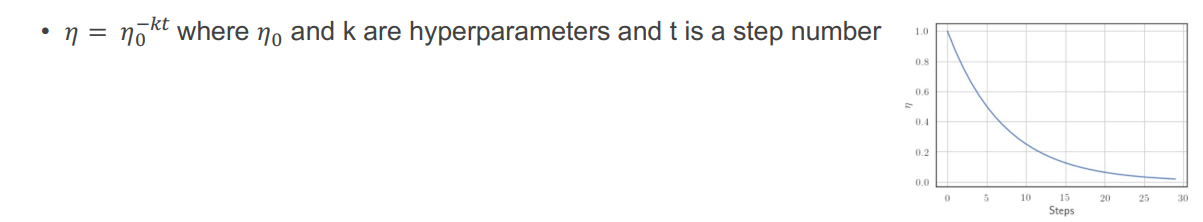
Exponential decay
Local minima
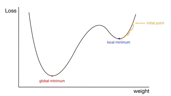
- 그 주변에서 최솟값이라고 전체 Loss에서의 최솟값이 아님!!
- SGD말고 MGD에서 계산하면 ㄱㅊ
Momentum(관성)
- 특히 높은 곡률, 작지만 일관된 gradient 또는 noisy gradient에 직면하여 학습을 가속화하도록 설계됨
- 지속적으로 수렴 방향이 일치한다면, 더 큰 폭으로 수렴하게끔 한다
➡ 빠른 학습 속도, local minima 개선
🔑 이해를 돕는 해설
장점
: 수렴 속도 향상, 이상치에 대한 저항성
단점
: 하이퍼파리미터 설정, 지역 최솟값의 우회
Weight initialization
Activation functions
- gradient가 없어지는 현상으로 뉴런이 포화됨
ReLU(Rectified Linear Unit)
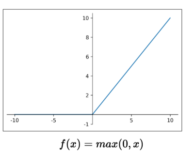
- 양수에서 포화되지 않음
- 컴퓨터적인 효율
- Sigmoid보다 수렴이 빠름(Gradient vanishing이 더 적게 일어남)
- 0보다 작은 것은 0으로, 0보다 큰 것은 1로 보는 방법
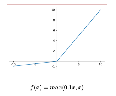
Leaky ReLU
- 위에서 발생하는 죽은 뉴런 문제를 해결하기 위해 고안된 방법
- 0보다 작을 때 기울기가 0이 아니기 때문에 뉴런이 지속적으로 업데이트 되어 죽는 것을 방지
Batch Normalization (BN)
Mini-batch SGD
QUIZ
- A single perceptron can solve nonlinear problems like the XOR problem (O/X)
- **For X with d=1 and output y<0, choose the update formula for w
- w=w+x
- w=w-x
- w=w*x
- w=w/x
- w=w(1-x)**
- For linearly separable binary data, the perceptron learning algorithm can obtain the weight vector w with a finite number of updates (O/X)
- Most real-world data is not linearly separable and contains many outliers, necessitating the use of MLPs to deal with such data and to find weights that minimize the error (O/X)
- A perceptron composed of an input layer and an output layer can be considered as a 2-layer MLP (O/X)
- When finding optimal weights in MLP, using a random guess is an effective method initially (O/X)
- The sigmoid function is more suitable as an activation function than the step function because it can have a wider range of output values (O/X)
- MLPs cannot solve multi-class classification problems (O/X)
- Choose back propagation method that divides the data into small parts and uses some of it for training. (SGD/BGD/MGD)
- For classification problem (number of class: K), the softmax output y is probability that input x belongs to each class → O
- MSE loss function이 Cross Entropy보다 더 수렴을 잘 한다 ⇒ X
- Deep learning process with multiple layers, final output contains the most relevant features and noise is filtered out → O
- When solving a task with sufficient data, a deeper network requires more neurons than a shallow network.→X
- When there is no activation function, the MLP is just learning linear transformation of input data → O(MLP는 비선형 문제 못 풀어서 Sigmoid 도입, 근데 Sigmoid가 activation)
- What happen when we initialize the weight with high values? → neurons will satureate very quickly
- For better convergence, we need to do finer search of learning rate → O
- What are the methods to achieve better convergence without falling into local minima? → Use momentum
Deep Learning
What is Deep Learning?
Deep vs Shallow
- 넓고 얕은 게(Shallow) 더 많은 hidden 뉴런을 필요로 함(더 많은 computation power 및 연산 필요)
- 깊이(Depth)는 상위 레이어에서 상대적으로 추상적인 개념들을 추상화 할 수 있는 가능성을 준다(충분한 데이터가 있다는 가정)
- 한 레이어는 통계를 탐지할 수 있지만 더 많은 뉴런을 필요로 함(다른 뉴런에 의존 불가능하기 때문)
왜 MLP는 이전에 DEEPLY 학습될 수 없었나?
1. 알고리즘 문제(Gradient vanashing, Poor initalization)
2. 컴퓨터가 너무 느림
3. 데이터 크기가 너무 작다
Algorithm Problem
Gradient vanashing
: x가 너무 커지거나 작아지면 gradient 값이 없어지는데 이를 gradient vanashing이라고 말한다.
Sigmoid activation function
: 뉴런이 포화되면, 기울기의 흐름이 없어짐
왜 뉴런이 포화될까? → 인풋은 0~1 사이에서 정규화됨
sigmoid 뉴런 사용 및 매우 높은 값으로 가중치를 초기화할 때 어떤일이 일어날까? → 뉴런들은 매우 빠르게 포화된다
한 레이어에 있는 수 백개의 뉴런들을 고려 → 가중치 합하면 2,3에 닿을 거임
Poor initialization
: 0으로 초기화하면(w=0) → a=0 → gradient가 동일해짐, 한번 망가지면 안 고쳐짐 = symmetry breaking problem
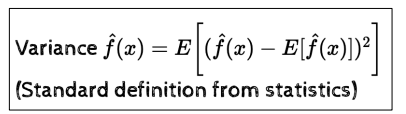
Bias-Variance Tradeoff
- (x,y) 점이 주어졌을 때 f를 예측
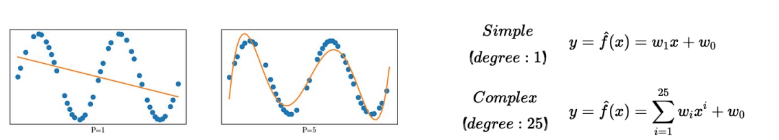
Simple Model
- 장점: 각각의 모델 간의 차이가 크지 않음
- 단점: 원하는 데이터의 개형을 예측하는 게 힘들다(under fitting)
Complex Model
- 장점: 심플 모델보다 더 정확하게 예측 가능
- 단점: 다른 데이터 샘플로 훈련된 복잡한 모델들은 서로 다른 모양을 가짐(high variance)
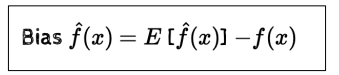
- bias = model의 평균 값과 실제 값의 차이
- Simple Model의 bias가 더 큼(complex model 보다)
- 모델 간 서로 얼마나 다른지
- Complex Model이 Simple Model보다 더 큰 variance를 가진다.
Simple Model: high bias, low variance
Complex Model: low bias, high variance 반대되는 경향을 가진다.
→ 서로 반대되는 경향을 가진다
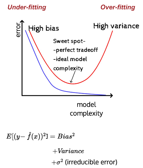
- train err: model complexity가 높아질 수록 점점 최적의 값이 됨
- test err: 내려오다 어느 순간부터 올라감
bias variance tradeoff와 model complexity를 고려해야 하는 이유
- DNN(Deep Neural Networks)는 highly complex model이다
- 많은 입력 값(parameter) => 주로 비선형
- overfit 하는 건 쉽지만 error를 0으로 만드는 건 어려움
- 따라서, 우리는 regularization이 필요하다
Regularization
-> test error를 줄이기 위한 전략(학습 오류 증가를 희생하여)
- L1/L2 Regularization
- Dataset augmentation
- Parameter Sharing and tying
- Early stopping
- Ensemble methods
- Dropout
L1/L2 normalization
L1 normalization
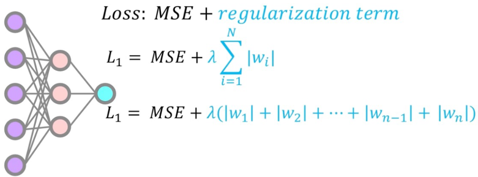
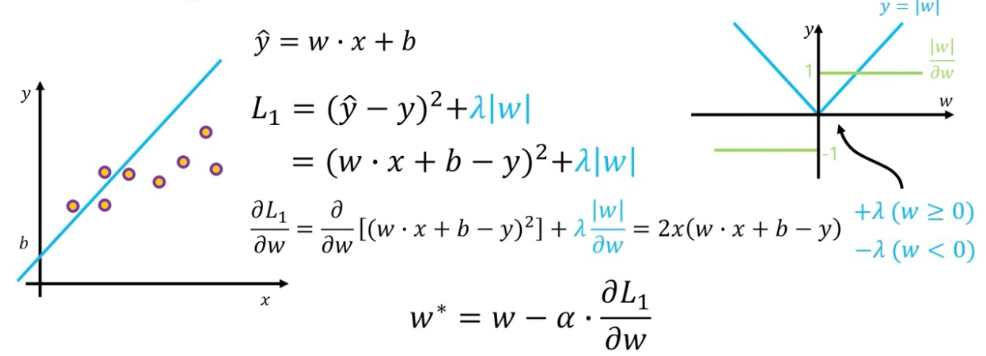
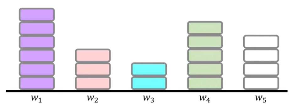
- 모든 weight가 0으로 가는 것보다 불필요한 weight가 거의 0에 수렴하여 영향력이 거의 없게함
- Model Complexity를 낮추기 위함 -> Model들의 complexity가 너무 크면 bias, variance로 인해 test error가 높아지니깐
L2 normalization
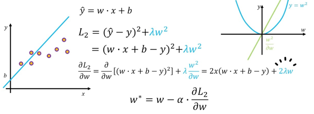
- w를 제곱해준다
- L1에 비해 더 안정적으로 weight 조절 가능
Enriching training data
- overfitting 할 수 있게 많은 고퀄리티 학습 데이터가 있으면 좋지만 현실적으로 어려움
Data augmentation(Label-preserving)
- 많은 데이터 => 좋은 학습 가능
- 하나의 값을 유지한 채 데이터를 불린다
- ex.) (x, y) => (x', y)
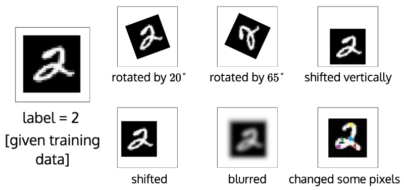
- ex.) (x, y) => (x', y)
Data augmentation(Label-perturbing)
- 일정 비율에 맞춰 데이터 값을 조절함
- x,y 둘 다 변형
- ex.) (x, y) => (x', y')
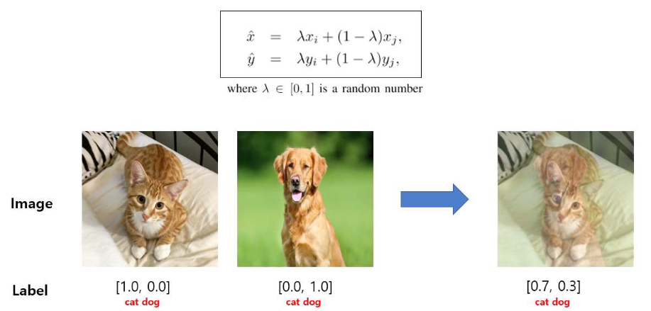
- ex.) (x, y) => (x', y')
좋은 모델보다 고퀄리티의 많은 data가 좋다
Parameter Sharing & Tying
- CNN에서 사용
- 이미지의 같은 위치에 같은 필터를 적용
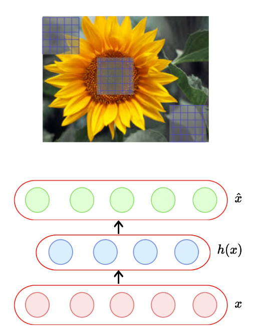
- 자동인코더에서 주로 사용
- 인코더와 디코더 weights는 묶여있다.
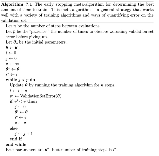
Early stopping
- MSE 같은 loss function을 0에 가깝도록 한다.
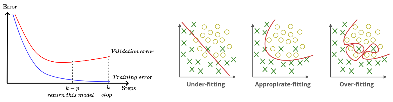
- 언제 멈춰야 할까
Ensembles
- 다른 샘플로 각 모델들을 학습한다.
- Bagging: 같은 분류기의 다른 인스턴스를 이용해 합침
- 한 모델의 다른 체크포인트들
- 다양성은 부족할 수있으나 합리적인 방식
- 이 접근은 매우 싸다
- 같은 모델, 다른 초기화
- ensemble을 만드는 거대 뉴런 네트워크 학습은 비싸다
- 옵션 1: 다른 아키텍쳐를 가진 뉴런 네트워크 학습
- 옵션 2: 다른 학습 샘플을 가지고 같은 네트워크 학습
- 옵션 1 또는 옵션 2를 사용하여 훈련하더라도 테스트 시간에 여러 모델을 결합하는 것은 실시간으론 불가능
Dropout
- Dropout은 이 문제들을 모두 해결하는 기술
- computational overhead 없이 뉴런 네트워크 학습
- 효과적인 근사 방법(지수적으로 많은 다른 네트워크들을 묶는 데)
- 뉴런 레벨에서의 정규화
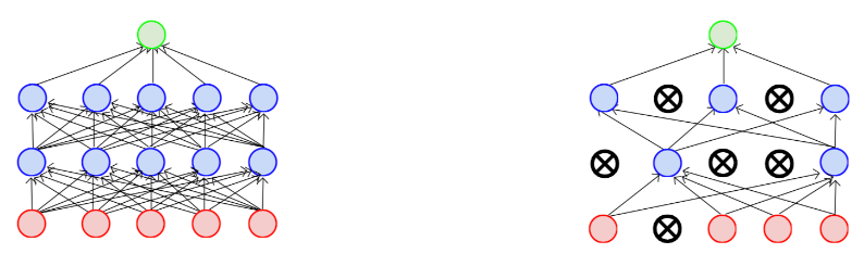
- 일시적으로 노드 및 모든 수신/발신 연결을 제거하여 네트워크가 얇아짐
- 각 노드는 고정된 확률로 유지(일반적으로 p=0.5)
- 각 노드를 유지하거나 드롭할 수 있습니다
N개 노드가 주어졌을 때, 얇은 네트워크가 형성될 수 있는 총 개수?
- 모든 네트워크 교차한 가중치 공유
- 각 학습 인스턴스의 다른 네트워크 샘플링
- 네트워크의 모든 파라미터(가중치)를 초기화 하고 학습 시작
- 첫 학습 인스턴스에서 dropout을 하여 얇은 네트워크 형성
- loss와 backpropagate 계산
- 두 번째 학습 인스턴스에서 dropout하여 다른 얇은 네트워크 형성
- 다시 loss와 backpropagate 계산
- weight가 하나의 학습 인스턴스에서만 활성화 됐다면 한 번만 업데이트 받았을 거임
- 만약 weight가 두 학습 인스턴에서 활성화 됐다면 두 번 업데이트 됐음
- 각 학습된 네트워크는 거의 학습되지 않지만 매개변수 공유를 통해 어떤 모델도 학습되지 않거나 제대로 학습되지 않은 매개변수가 없도록 보장합니다
- Dropout은 필수적으로 hidden unit에 masking noise 적용
- hidden unit이 coadapting 되는 것 방지
- hidden unit이 언제든 dropout 될 수 있으므로 너무 의존할 수 없음
- 각 hidden unit이 random dropout에 대해 더 강력한 학습 필요
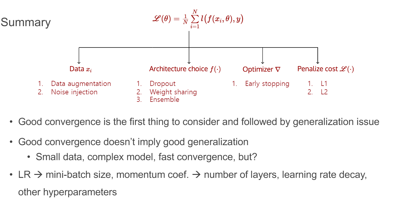
- 좋은 수렴이 첫 번째이고 정규화는 다음 문제
- 좋은 수렴은 좋은 정규화를 보장하지 않음
- 적은 데이터, 복잡한 모델, 빠른 수렴 등
- LR -> 작은 batch 크기, 모멘텀 -> 레이어의 수, 학습 속도 decay, 하이퍼파라미터 등