overview
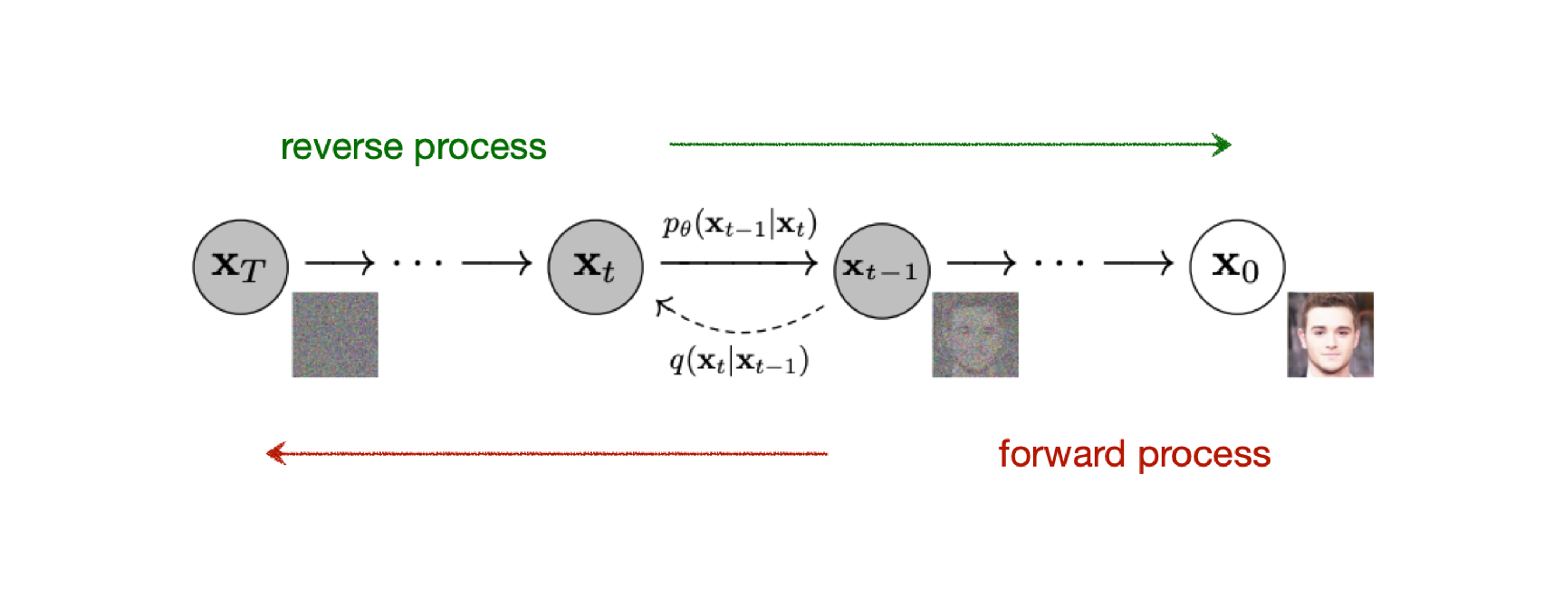
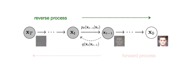
Diffusion model 은 위 그림에서 보면, x 0 \mathbf{x}_0 x 0 x T \mathbf{x}_T x T
noise 를 계속 더해가는 과정을 forward process q q q p θ p_{\theta} p θ
이를 통해서 실제 data 의 분포인 p ( x 0 ) p(\mathbf{x}_0) p ( x 0 )
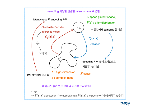
latent space z 가 noise 라는거군, 근데 이게 gaussian 으로 되니까 일반적인 VAE
Forward process
원본 이미지 x 0 \mathbf{x}_0 x 0 x T \mathbf{x}_T x T x T \mathbf{x}_T x T 0 0 0
이미지 x t − 1 \mathbf{x}_{t-1} x t − 1 β t \beta_t β t x t \mathbf{x}_t x t q q q ϵ t − 1 \epsilon_{t-1} ϵ t − 1 0 0 0
x t = 1 − β t x t − 1 + β t ϵ t − 1 \mathbf{x}_{t} = \sqrt{1-\beta_t}\mathbf{x}_{t-1} + \sqrt{\beta_t}\epsilon_{t-1} x t = 1 − β t x t − 1 + β t ϵ t − 1 입력 이미지 x t − 1 \mathbf{x}_{t-1} x t − 1 x t \mathbf{x}_t x t x 0 \mathbf{x}_0 x 0 0 0 0 T T T x T \mathbf{x}_T x T
x t − 1 \mathbf{x}_{t-1} x t − 1 0 0 0 ( I ) (I) ( I ) V a r ( a X ) = a 2 V a r ( X ) Var(aX) = a^2Var(X) V a r ( a X ) = a 2 V a r ( X )
V a r ( 1 − β t x t − 1 ) = ( 1 − β t ) I = 1 − β t V a r ( β t ϵ t − 1 ) = β I = β \begin{aligned} Var \left(\sqrt{1-\beta_t}\mathbf{x}_{t-1}\right) &= \left( 1-\beta_t \right)I = 1-\beta_t \\ Var(\sqrt{\beta_t}\epsilon_{t-1}) &= \beta I = \beta \end{aligned} V a r ( 1 − β t x t − 1 ) V a r ( β t ϵ t − 1 ) = ( 1 − β t ) I = 1 − β t = β I = β 여기서 1 − β t x t − 1 \sqrt{1-\beta_t}\mathbf{x}_{t-1} 1 − β t x t − 1 β t ϵ t − 1 \sqrt{\beta_t}\epsilon_{t-1} β t ϵ t − 1 X , Y X, Y X , Y V a r ( X + Y ) = V a r ( X ) + V a r ( Y ) Var(X + Y) = Var(X) + Var(Y) V a r ( X + Y ) = V a r ( X ) + V a r ( Y )
이 둘을 합치면 평균이 0 0 0 1 − β t + β t = 1 1-\beta_t + \beta_t = 1 1 − β t + β t = 1 x t \mathbf{x}_t x t
따라서 x 0 \mathbf{x}_0 x 0 0 0 0 x T \mathbf{x}_T x T x t \mathbf{x}_t x t
간단히 x t \mathbf{x}_t x t q q q
q ( x t ∣ x t − 1 ) = N ( x t ; 1 − β t x t − 1 , β t I ) q(\mathbf{x}_t|\mathbf{x}_{t-1}) = \mathcal{N}(\mathbf{x}_{t}; \sqrt{1-\beta_t} \mathbf{x}_{t-1}, \beta_t I) q ( x t ∣ x t − 1 ) = N ( x t ; 1 − β t x t − 1 , β t I ) Reparameterization trick
q q q t t t x 0 \mathbf{x}_0 x 0 x t \mathbf{x}_t x t
α t = 1 − β t \alpha_t = 1-\beta_t α t = 1 − β t α ˉ t = ∏ i = 1 t α i \bar{\alpha}_t = \prod^{t}_{i=1} \alpha_i α ˉ t = ∏ i = 1 t α i
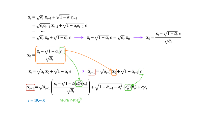
x t = α t x t − 1 + 1 − α t ϵ t − 1 = α t α t − 1 x t − 2 + 1 − α t α t − 1 ϵ = ⋯ = α ˉ t x 0 + 1 − α t ˉ ϵ \begin{aligned} \mathbf{x}_t &= \sqrt{\alpha_t} \; \mathbf{x}_{t-1} + \sqrt{1-\alpha_t}\; \epsilon_{t-1} \\ &= \sqrt{\alpha_t \alpha_{t-1}} \; \mathbf{x}_{t-2} + \sqrt{1-\alpha_t\alpha_{t-1}}\;\epsilon \\ &= \quad \cdots \\ &= \sqrt{\bar{\alpha}_t}\;\mathbf{x}_0 + \sqrt{1-\bar{\alpha_t}}\;\epsilon \end{aligned} x t = α t x t − 1 + 1 − α t ϵ t − 1 = α t α t − 1 x t − 2 + 1 − α t α t − 1 ϵ = ⋯ = α ˉ t x 0 + 1 − α t ˉ ϵ 두 번째 줄은 두 개의 gaussian dist 를 더하여 새로운 gaussian dist 하나를 얻을 수 있다는 사실을 이용하였다. 좀 더 수식을 명확히 해보자.
q ( x 1 : T ∣ x 0 ) = ∏ t = 1 T q ( x t ∣ x t − 1 ) , q ( x t ∣ x t − 1 ) = N ( x t ; 1 − β t x t − 1 , β t I ) q(\mathbf{x}_{1:T}|\mathbf{x}_0) = \prod^{T}_{t=1}q(\mathbf{x}_t|\mathbf{x}_{t-1}), \quad q(\mathbf{x}_t|\mathbf{x}_{t-1}) = \mathcal{N}(\mathbf{x}_{t}; \sqrt{1-\beta_t} \mathbf{x}_{t-1}, \beta_t I) q ( x 1 : T ∣ x 0 ) = t = 1 ∏ T q ( x t ∣ x t − 1 ) , q ( x t ∣ x t − 1 ) = N ( x t ; 1 − β t x t − 1 , β t I ) normal distribution 의 가법성에 따라 독립인 두 확률 변수는
X ∼ N ( μ x , σ x 2 ) , Y ∼ N ( μ y , σ y 2 ) X \sim \mathcal{N}\left( \mu_x, \sigma^{2}_{x} \right), \quad Y \sim \mathcal{N}\left( \mu_y, \sigma^{2}_{y} \right) X ∼ N ( μ x , σ x 2 ) , Y ∼ N ( μ y , σ y 2 ) 를 더하면
Z ∼ N ( μ x + μ y , σ x 2 + σ y 2 ) Z \sim \mathcal{N} \left( \mu_x + \mu_y, \sigma^{2}_{x} + \sigma^{2}_{y} \right) Z ∼ N ( μ x + μ y , σ x 2 + σ y 2 ) 따라서, 첫 번째 줄의 x t − 1 \mathbf{x}_{t-1} x t − 1 x t − 2 \mathbf{x}_{t-2} x t − 2
x t = α t x t − 1 + 1 − α ϵ t − 1 = α t ( α t − 1 x t − 2 + 1 − α t − 1 ϵ t − 2 ) + 1 − α t ϵ t − 1 = α t α t − 1 x t − 2 + α t ( 1 − α t − 1 ) ϵ t − 2 + 1 − α t ϵ t − 1 = α t α t − 1 x t − 2 + α t ( 1 − α t − 1 ) + 1 − α t ϵ = α t α t − 1 x t − 2 + 1 − α t α t − 1 ϵ \begin{aligned} \mathbf{x}_t &= \sqrt{\alpha_{t}}\;\mathbf{x}_{t-1} + \sqrt{1-\alpha} \; \epsilon_{t-1} \\ &= \sqrt{\alpha_t}(\sqrt{\alpha_{t-1}}\;\mathbf{x}_{t-2} + \sqrt{1-\alpha_{t-1}}\;\epsilon_{t-2}) + \sqrt{1-\alpha_t}\;\epsilon_{t-1} \\ &= \sqrt{\alpha_t \alpha_{t-1}}\;\mathbf{x}_{t-2} + \sqrt{\alpha_t(1-\alpha_{t-1})}\;\epsilon_{t-2} + \sqrt{1-\alpha_{t}}\;\epsilon_{t-1} \\ &= \sqrt{\alpha_t \alpha_{t-1}}\;\mathbf{x}_{t-2} + \sqrt{\alpha_t(1-\alpha_{t-1}) + 1-\alpha_t} \; \epsilon \\ &= \sqrt{\alpha_t \alpha_{t-1}}\;\mathbf{x}_{t-2} + \sqrt{1-\alpha_t\alpha_{t-1}}\;\epsilon \end{aligned} x t = α t x t − 1 + 1 − α ϵ t − 1 = α t ( α t − 1 x t − 2 + 1 − α t − 1 ϵ t − 2 ) + 1 − α t ϵ t − 1 = α t α t − 1 x t − 2 + α t ( 1 − α t − 1 ) ϵ t − 2 + 1 − α t ϵ t − 1 = α t α t − 1 x t − 2 + α t ( 1 − α t − 1 ) + 1 − α t ϵ = α t α t − 1 x t − 2 + 1 − α t α t − 1 ϵ 따라서 원본 이미지 x 0 \mathbf{x}_0 x 0
또한 원래 β t \beta_t β t α t ˉ \bar{\alpha_t} α t ˉ ( ϵ ) (\epsilon) ( ϵ ) q q q
q ( x t ∣ x 0 ) = N ( x t ; α ˉ x 0 , ( 1 − α t ˉ ) I ) q(\mathbf{x}_t|\mathbf{x}_0) = \mathcal{N}(\mathbf{x}_t; \sqrt{\bar{\alpha}}\;\mathbf{x}_0,\; (1-\bar{\alpha_t})I) q ( x t ∣ x 0 ) = N ( x t ; α ˉ x 0 , ( 1 − α t ˉ ) I ) Reverse process
noise 추가 과정을 되돌릴 수 있는 신경망 p θ ( x t − 1 ∣ x t ) p_{\theta}(\mathbf{x}_{t-1}|\mathbf{x}_t) p θ ( x t − 1 ∣ x t ) q ( x t ∣ x t − 1 ) q(\mathbf{x}_{t}|\mathbf{x}_{t-1}) q ( x t ∣ x t − 1 ) p θ ( x t − 1 ∣ x t ) p_{\theta}(\mathbf{x}_{t-1}|\mathbf{x}_t) p θ ( x t − 1 ∣ x t ) x T \mathbf{x}_T x T x 0 \mathbf{x}_0 x 0
이렇게 할 수 있다면 N ( 0 , I ) \mathcal{N}(0, I) N ( 0 , I )
Reverse process 와 Variational AutoEncoder(VAE) 의 decoder 사이에는 많은 유사점이 있다. 두 모델 모두 신경망을 사용하여 random 한 noise 를 의미 있는 출력으로 변환하는 것이 목표.
diffusion model 과 VAE 의 차이는 VAE 에서는 forward process (이미지를 noise 로 변환) 가 모델의 일부이지만, diffusion model 에서는 이에 대한 parameter 가 없다. BaseVAE 모델의 code review link 를 보면 Encoder, Decoder 가 있지만, diffusion model 은 같은 모델을 사용한다.
diffusion model 이 실제로는 두 개의 신경망 복사본을 유지한다.
gradient descent 를 사용하여 훈련된 신경망
이전 훈련 단계에서 훈련된 신경망 weight 의 exponential moving average (EMA) 를 사용하는 신경망 (EMA 신경망)
이다.
EMA 신경망은 훈련 과정에서 단기적인 변동과 등락에 영향을 받지 않으므로 능동적으로 훈련된 신경망보다 더 안정적으로 생성 작업을 수행한다. 따라서 신경망으로 출력을 생성할 때 EMA 신경망을 사용한다.
Algorithm 1
1: repeat x 0 ∼ q ( x 0 ) \mathbf{x}_0 \sim q(\mathbf{x}_0) x 0 ∼ q ( x 0 ) t ∼ t \sim t ∼ ( { 1 , ⋯ , T } ) (\{1, \cdots, T\}) ( { 1 , ⋯ , T } ) ϵ ∼ N ( 0 , I ) \epsilon \sim \mathcal{N}(\mathbf{0}, \mathbf{I}) ϵ ∼ N ( 0 , I )
▽ θ ∥ ϵ − ϵ θ ( α t ˉ x 0 + 1 − α t ˉ ϵ , t ) ∥ 2 \bigtriangledown_{\theta} \parallel \epsilon - \epsilon_{\theta}( \sqrt{\bar{\alpha_t}}\mathbf{x}_0 + \sqrt{1-\bar{\alpha_t}}\;\epsilon , t)\parallel^2 ▽ θ ∥ ϵ − ϵ θ ( α t ˉ x 0 + 1 − α t ˉ ϵ , t ) ∥ 2 6: until converged
noise 제거 diffusion model 의 훈련 과정.
random noise 에서 data 를 복원하는 모델로 사용되기 때문에 diffusion model 을 사용하기 위해서는 modeling 하는 것이 필수적이지만, 이것을 실제로 알아내는 것은 쉽지 않다. 원래 decoding 이 어렵다.
Reverse process 의 시작점인 noise 의 분포는
p ( x T ) = N ( x T ; 0 , I ) p(\mathbf{x}_T) = \mathcal{N}(\mathbf{x}_T;\mathbf{0}, I) p ( x T ) = N ( x T ; 0 , I ) noise 의 분포가 된다.
그리고 p θ p_{\theta} p θ
p θ ( x 0 : T ) : = p ( x T ) ∏ t = 1 T p θ ( x t − 1 ∣ x t ) , p θ ( x t − 1 ∣ x t ) : = N ( x t − 1 ; μ θ ( x t , t ) , Σ θ ( x t , t ) ) \begin{aligned} p_\theta(\mathbf{x}_{0:T}) &:= p(\mathbf{x}_T)\prod^{T}_{t=1}p_{\theta}(\mathbf{x}_{t-1}|\mathbf{x}_t), \\ p_{\theta}(\mathbf{x}_{t-1}|\mathbf{x}_t) &:= \mathcal{N}(\mathbf{x}_{t-1};\mu_\theta(\mathbf{x}_{t}, t), \Sigma_{\theta}(\mathbf{x}_t, t)) \end{aligned} p θ ( x 0 : T ) p θ ( x t − 1 ∣ x t ) : = p ( x T ) t = 1 ∏ T p θ ( x t − 1 ∣ x t ) , : = N ( x t − 1 ; μ θ ( x t , t ) , Σ θ ( x t , t ) ) reverse process 의 수식 표현.
위 식에서, 각 단계의 normal distribution 의 평균 μ θ \mu_\theta μ θ Σ θ \Sigma_{\theta} Σ θ
Training (Loss function)
encoder, decoder 의 로직은 확인했고, training 을 위한 loss function 을 확인해보자. p θ p_{\theta} p θ p ( x 0 ) p(\mathbf{x}_0) p ( x 0 )
Ref. paper eq.2-(3) (p.2)
E [ − log p θ ( x 0 ) ] ≤ E q [ − log p θ ( x 0 : T ) q ( x 1 : T ∣ x 0 ) ] = E q [ − log p ( x T ) − ∑ t ≥ 1 log p θ ( x t − 1 ∣ x t ) q ( x t ∣ x t − 1 ) ] : = L \begin{aligned} \mathbb{E}\left[-\log p_{\theta}(\mathbf{x}_0)\right] &\leq \mathbb{E}_q \left[ -\log\frac{p_{\theta}(\mathbf{x}_{0:T})}{q(\mathbf{x}_{1:T}|\mathbf{x}_0)}\right] \\ &= \mathbb{E}_{q} \left[ -\log p(\mathbf{x}_T) - \sum_{t \geq 1} \log \frac{p_{\theta}(\mathbf{x}_{t-1}|\mathbf{x}_t)}{q(\mathbf{x}_t|\mathbf{x}_{t-1})}\right] := L \end{aligned} E [ − log p θ ( x 0 ) ] ≤ E q [ − log q ( x 1 : T ∣ x 0 ) p θ ( x 0 : T ) ] = E q [ − log p ( x T ) − t ≥ 1 ∑ log q ( x t ∣ x t − 1 ) p θ ( x t − 1 ∣ x t ) ] : = L 위 식의 두 번째 부등호는 다음과 같이 증명할 수 있다.
− log p θ ( x 0 ) ≤ − log p θ ( x 0 ) + D K L ( q ( x 1 : T ∣ x 0 ) ∣ ∣ p θ ( x 1 : T ∣ x 0 ) ) = − log p θ ( x 0 ) + E x 1 : T ∼ q ( x 1 : T ∣ x 0 ) [ log q ( x 1 : T ∣ x 0 ) p θ ( x 0 : T ) / p θ ( x 0 ) ] = − log p θ ( x 0 ) + E q [ log q ( x 1 : T ∣ x 0 ) p θ ( x 0 : T ) + log p θ ( x 0 ) ] = E q [ log q ( x 1 : T ∣ x 0 ) p θ ( x 0 : T ) ] − log p θ ( x 0 ) ≤ E q [ − log p θ ( x 0 : T ) q ( x 1 : T ∣ x 0 ) ] \begin{aligned} -\log p_{\theta}(\mathbf{x}_0) & \leq -\log p_{\theta}(\mathbf{x}_0) + D_{KL}(q(\mathbf{x}_{1:T}|\mathbf{x}_0)||p_{\theta}(\mathbf{x}_{1:T}|\mathbf{x}_0)) \\ &= -\log p_{\theta}(\mathbf{x}_0) + \mathbb{E}_{\mathbf{x}_{1:T} \sim q(\mathbf{x}_{1:T}|\mathbf{x}_0)} \left[ \log \frac{q(\mathbf{x}_{1:T}|\mathbf{x}_0)}{p_{\theta}(\mathbf{x}_{0:T})/p_\theta(\mathbf{x}_0)} \right] \\ &= -\log p_{\theta}(\mathbf{x}_0) + \mathbb{E}_q \left[\log \frac{q(\mathbf{x}_{1:T}|\mathbf{x}_0)}{p_{\theta}(\mathbf{x}_{0:T})} + \log p_{\theta}(\mathbf{x}_0)\right] \\ &= \mathbb{E}_q \left[\log \frac{q(\mathbf{x}_{1:T}|\mathbf{x}_0)}{p_{\theta}(\mathbf{x}_{0:T})}\right] \\ -\log{p_{\theta}}(\mathbf{x}_{0}) &\leq \mathbb{E}_q \left[-\log \frac{p_{\theta}(\mathbf{x}_{0:T})}{q(\mathbf{x}_{1:T}|\mathbf{x}_0)}\right] \end{aligned} − log p θ ( x 0 ) − log p θ ( x 0 ) ≤ − log p θ ( x 0 ) + D K L ( q ( x 1 : T ∣ x 0 ) ∣ ∣ p θ ( x 1 : T ∣ x 0 ) ) = − log p θ ( x 0 ) + E x 1 : T ∼ q ( x 1 : T ∣ x 0 ) [ log p θ ( x 0 : T ) / p θ ( x 0 ) q ( x 1 : T ∣ x 0 ) ] = − log p θ ( x 0 ) + E q [ log p θ ( x 0 : T ) q ( x 1 : T ∣ x 0 ) + log p θ ( x 0 ) ] = E q [ log p θ ( x 0 : T ) q ( x 1 : T ∣ x 0 ) ] ≤ E q [ − log q ( x 1 : T ∣ x 0 ) p θ ( x 0 : T ) ] 두 번째 부등호의 증명 Q.E.D.
위 식의 세 번째 등호는
Forward process
q ( x 1 : T ∣ x 0 ) = ∏ t = 1 T q ( x t ∣ x t − 1 ) , q ( x t ∣ x t − 1 ) = N ( x t ; 1 − β t x t − 1 , β t I ) q(\mathbf{x}_{1:T}|\mathbf{x}_0) = \prod^{T}_{t=1}q(\mathbf{x}_t|\mathbf{x}_{t-1}), \quad q(\mathbf{x}_t|\mathbf{x}_{t-1}) = \mathcal{N}(\mathbf{x}_{t}; \sqrt{1-\beta_t} \mathbf{x}_{t-1}, \beta_t I) q ( x 1 : T ∣ x 0 ) = t = 1 ∏ T q ( x t ∣ x t − 1 ) , q ( x t ∣ x t − 1 ) = N ( x t ; 1 − β t x t − 1 , β t I )
Reverse process
p θ ( x 0 : T ) : = p ( x T ) ∏ t = 1 T p θ ( x t − 1 ∣ x t ) , p θ ( x t − 1 ∣ x t ) : = N ( x t − 1 ; μ θ ( x t , t ) , Σ θ ( x t , t ) ) \begin{aligned} p_\theta(\mathbf{x}_{0:T}) &:= p(\mathbf{x}_T)\prod^{T}_{t=1}p_{\theta}(\mathbf{x}_{t-1}|\mathbf{x}_t), \\ p_{\theta}(\mathbf{x}_{t-1}|\mathbf{x}_t) &:= \mathcal{N}(\mathbf{x}_{t-1};\mu_\theta(\mathbf{x}_{t}, t), \Sigma_{\theta}(\mathbf{x}_t, t)) \end{aligned} p θ ( x 0 : T ) p θ ( x t − 1 ∣ x t ) : = p ( x T ) t = 1 ∏ T p θ ( x t − 1 ∣ x t ) , : = N ( x t − 1 ; μ θ ( x t , t ) , Σ θ ( x t , t ) )
log \log log
E q [ − log p θ ( x 0 : T ) q ( x 1 : T ∣ x 0 ) ] = E q [ − log p ( x T ) − ∑ t ≥ 1 log p θ ( x t − 1 ∣ x t ) q ( x t ∣ x t − 1 ) ] : = L \mathbb{E}_q \left[ -\log\frac{p_{\theta}(\mathbf{x}_{0:T})}{q(\mathbf{x}_{1:T}|\mathbf{x}_0)}\right] = \mathbb{E}_{q} \left[ -\log p(\mathbf{x}_T) - \sum_{t \geq 1} \log \frac{p_{\theta}(\mathbf{x}_{t-1}|\mathbf{x}_t)}{q(\mathbf{x}_t|\mathbf{x}_{t-1})}\right] := L E q [ − log q ( x 1 : T ∣ x 0 ) p θ ( x 0 : T ) ] = E q [ − log p ( x T ) − t ≥ 1 ∑ log q ( x t ∣ x t − 1 ) p θ ( x t − 1 ∣ x t ) ] : = L 등호의 증명 Q.E.D.
이 식을, KL-Divergence 형태로 변형하여 loss function 으로 사용하기 좋게 만들 수 있다.
Ref. paper Appendix A (p.13)
L = E q [ − log p θ ( x 0 : T ) q ( x 1 : T ∣ x 0 ) ] = E q [ − log p ( x T ) − ∑ t ≥ 1 log p θ ( x t − 1 ∣ x t ) q ( x t ∣ x t − 1 ) ] = E q [ − log p ( x T ) − ∑ t > 1 log p θ ( x t − 1 ∣ x t ) q ( x t ∣ x t − 1 ) − log p θ ( x 0 ∣ x 1 ) q ( x 1 ∣ x 0 ) ] = E q [ − log p ( x T ) − ∑ t > 1 log ( p θ ( x t − 1 ∣ x t ) q ( x t − 1 ∣ x t , x 0 ) ⋅ q ( x t − 1 ∣ x 0 ) q ( x t ∣ x 0 ) ) − log p θ ( x 0 ∣ x 1 ) q ( x 1 ∣ x 0 ) ] = E q [ − log p ( x T ) q ( x T ∣ x 0 ) − ∑ t > 1 log p θ ( x t − 1 ∣ x t ) q ( x t − 1 ∣ x t , x 0 ) − log p θ ( x 0 ∣ x 1 ) ] = E q [ D K L ( q ( x T ∣ x 0 ) ∥ p ( x T ) ) + ∑ t > 1 D K L ( q ( x t − 1 ∣ x t , x 0 ) ∥ p θ ( x t − 1 ∣ x t ) ) − log p θ ( x 0 ∣ x 1 ) ] \begin{aligned} L &= \mathbb{E}_q \left[ -\log\frac{p_{\theta}(\mathbf{x}_{0:T})}{q(\mathbf{x}_{1:T}|\mathbf{x}_0)}\right] \\ &= \mathbb{E}_{q} \left[ -\log p(\mathbf{x}_T) - \sum_{t \geq 1} \log \frac{p_{\theta}(\mathbf{x}_{t-1}|\mathbf{x}_t)}{q(\mathbf{x}_t|\mathbf{x}_{t-1})}\right] \\ &= \mathbb{E}_q \left[ -\log p(\mathbf{x}_T) - \sum_{t > 1} \log \frac{p_{\theta}(\mathbf{x}_{t-1}|\mathbf{x}_t)}{q(\mathbf{x}_t|\mathbf{x}_{t-1})} - \log \frac{p_{\theta}(\mathbf{x}_0|\mathbf{x}_1)}{q(\mathbf{x}_1|\mathbf{x}_0)} \right] \\ &= \mathbb{E}_q \left[ -\log p(\mathbf{x}_T) - \sum_{t > 1} \log \left( \frac{p_{\theta}(\mathbf{x}_{t-1}|\mathbf{x}_t)}{q(\mathbf{x}_{t-1}|\mathbf{x}_t, \mathbf{x}_0)} \cdot \frac{q(\mathbf{x}_{t-1}|\mathbf{x}_0)}{q(\mathbf{x}_t|\mathbf{x}_0)} \right) - \log \frac{p_{\theta}(\mathbf{x}_0|\mathbf{x}_1)}{q(\mathbf{x}_1|\mathbf{x}_0)} \right] \\ &= \mathbb{E}_q \left[ -\log \frac{p(\mathbf{x}_T)}{q(\mathbf{x}_T|\mathbf{x}_0)} - \sum_{t > 1} \log \frac{p_{\theta}(\mathbf{x}_{t-1}|\mathbf{x}_t)}{q(\mathbf{x}_{t-1}|\mathbf{x}_t, \mathbf{x}_0)}- \log p_{\theta}(\mathbf{x}_0|\mathbf{x}_1) \right] \\ &= \mathbb{E}_q \left[D_{KL}(q(\mathbf{x}_T|\mathbf{x}_0) \; \Vert \; p(\mathbf{x}_T)) + \sum_{t > 1}D_{KL}(q(\mathbf{x}_{t-1}|\mathbf{x}_t, \mathbf{x}_0) \; \Vert \; p_{\theta}(\mathbf{x}_{t-1}|\mathbf{x}_t))- \log p_{\theta}(\mathbf{x}_0|\mathbf{x}_1) \right] \\ \; \\ \end{aligned} L = E q [ − log q ( x 1 : T ∣ x 0 ) p θ ( x 0 : T ) ] = E q [ − log p ( x T ) − t ≥ 1 ∑ log q ( x t ∣ x t − 1 ) p θ ( x t − 1 ∣ x t ) ] = E q [ − log p ( x T ) − t > 1 ∑ log q ( x t ∣ x t − 1 ) p θ ( x t − 1 ∣ x t ) − log q ( x 1 ∣ x 0 ) p θ ( x 0 ∣ x 1 ) ] = E q [ − log p ( x T ) − t > 1 ∑ log ( q ( x t − 1 ∣ x t , x 0 ) p θ ( x t − 1 ∣ x t ) ⋅ q ( x t ∣ x 0 ) q ( x t − 1 ∣ x 0 ) ) − log q ( x 1 ∣ x 0 ) p θ ( x 0 ∣ x 1 ) ] = E q [ − log q ( x T ∣ x 0 ) p ( x T ) − t > 1 ∑ log q ( x t − 1 ∣ x t , x 0 ) p θ ( x t − 1 ∣ x t ) − log p θ ( x 0 ∣ x 1 ) ] = E q [ D K L ( q ( x T ∣ x 0 ) ∥ p ( x T ) ) + t > 1 ∑ D K L ( q ( x t − 1 ∣ x t , x 0 ) ∥ p θ ( x t − 1 ∣ x t ) ) − log p θ ( x 0 ∣ x 1 ) ] Ref. paper Connection to autoregresive decoding (p.7 and p.14)L L L
L = D K L ( q ( x T ) ∥ p ( x T ) ) + E q [ ∑ t ≥ 1 D K L ( q ( x t − 1 ∣ x t ) ∥ p θ ( x t − 1 ∣ x t ) ) ] + H ( x 0 ) L = D_{KL}(q(\mathbf{x}_T) \; \Vert \; p(\mathbf{x}_T)) + \mathbb{E}_q \left[ \sum_{t \geq 1} D_{KL}(q(\mathbf{x}_{t-1}|\mathbf{x}_t) \; \Vert \; p_{\theta}(\mathbf{x}_{t-1}|\mathbf{x}_{t})) \right] + H(\mathbf{x}_0) L = D K L ( q ( x T ) ∥ p ( x T ) ) + E q [ t ≥ 1 ∑ D K L ( q ( x t − 1 ∣ x t ) ∥ p θ ( x t − 1 ∣ x t ) ) ] + H ( x 0 ) encoder : forward : q q q reverse : p θ p_\theta p θ
L T = D K L ( q ( x T ∣ x 0 ) ∥ p ( x T ) ) L_T = D_{KL}(q(\mathbf{x}_T|\mathbf{x}_0) \; \Vert \; p(\mathbf{x}_T)) L T = D K L ( q ( x T ∣ x 0 ) ∥ p ( x T ) ) → \rightarrow → x 0 \mathbf{x}_0 x 0 x t \mathbf{x}_t x t x t \mathbf{x}_t x t
L t − 1 = D K L ( q ( x t − 1 ∣ x t , x 0 ) ∥ p θ ( x t − 1 ∣ x t ) ) L_{t-1} = D_{KL}(q(\mathbf{x}_{t-1}|\mathbf{x}_t, \mathbf{x}_0) \; \Vert \; p_{\theta}(\mathbf{x}_{t-1}|\mathbf{x}_t)) L t − 1 = D K L ( q ( x t − 1 ∣ x t , x 0 ) ∥ p θ ( x t − 1 ∣ x t ) ) → \rightarrow →
L 0 = − log p θ ( x 0 ∣ x 1 ) L_0 = -\log p_{\theta}(\mathbf{x}_0|\mathbf{x}_1) L 0 = − log p θ ( x 0 ∣ x 1 ) → \rightarrow → x 1 \mathbf{x}_1 x 1 x 0 \mathbf{x}_0 x 0
q ( x t − 1 ∣ x t , x 0 ) = N ( x t − 1 ; μ ~ t ( x t , x 0 ) , β ~ t I ) , where μ ~ t ( x t , x 0 ) : = α ˉ t − 1 β t 1 − α ˉ t x 0 + α t ( 1 − α ˉ t − 1 ) 1 − α ˉ t x t a n d β ~ t : = 1 − α ˉ t − 1 1 − α ˉ t β t \begin{aligned} q(\mathbf{x}_{t-1}|\mathbf{x}_t, \mathbf{x}_0) &= \mathcal{N}(\mathbf{x}_{t-1}; \tilde{\mu}_t(\mathbf{x}_t, \mathbf{x}_0), \tilde{\beta}_t\mathbf{I}), \\ \text{where} \;\tilde{\mu}_t(\mathbf{x}_t, \mathbf{x}_0) &:= \frac{\sqrt{\bar{\alpha}_{t-1}}\beta_t}{1-\bar{\alpha}_t}\mathbf{x}_0 + \frac{\sqrt{\alpha_t}(1-\bar{\alpha}_{t-1})}{1-\bar{\alpha}_t}\mathbf{x}_t \quad {\rm and} \quad \tilde{\beta}_t:=\frac{1-\bar{\alpha}_{t-1}}{1-\bar{\alpha}_t}\beta_t \end{aligned} q ( x t − 1 ∣ x t , x 0 ) where μ ~ t ( x t , x 0 ) = N ( x t − 1 ; μ ~ t ( x t , x 0 ) , β ~ t I ) , : = 1 − α ˉ t α ˉ t − 1 β t x 0 + 1 − α ˉ t α t ( 1 − α ˉ t − 1 ) x t a n d β ~ t : = 1 − α ˉ t 1 − α ˉ t − 1 β t
q ( x t − 1 ∣ x t , x 0 ) q(\mathbf{x}_{t-1}|\mathbf{x}_t, \mathbf{x}_0) q ( x t − 1 ∣ x t , x 0 ) q ( x t − 1 ∣ x t , x 0 ) = q ( x t ∣ x t − 1 , x 0 ) q ( x t − 1 ∣ x 0 ) q ( x t ∣ x 0 ) ∝ exp ( − 1 2 ( ( x t − α t x t − 1 ) 2 β t + ( x t − 1 − α ˉ t − 1 x 0 ) 2 1 − α ˉ t − 1 − ( x t − α t x 0 ) 2 1 − α ˉ t ) ) = exp ( − 1 2 ( x t 2 − 2 α t x t x t − 1 + α t x t − 1 2 β t + x t − 1 2 − 2 α ˉ t − 1 x 0 x t − 1 + α ˉ t − 1 x 0 2 1 − α ˉ t − 1 − ( x t − α ˉ t x 0 ) 2 1 − α ˉ t ) ) = exp ( − 1 2 ( ( α t β t + 1 1 − α ˉ t − 1 ) x t − 1 2 − ( 2 α t β t x t + 2 α ˉ t − 1 1 − α ˉ t − 1 x 0 ) x t − 1 + C ( x t , x 0 ) ) ) \begin{aligned} q(\mathbf{x}_{t-1}|\mathbf{x}_t, \mathbf{x}_0) &= q(\mathbf{x}_t|\mathbf{x}_{t-1}, \mathbf{x}_0)\frac{q(\mathbf{x}_{t-1}|\mathbf{x}_0)}{q(\mathbf{x}_t|\mathbf{x}_0)} \\ &\propto \exp \left( -\frac{1}{2}\left( \frac{(\mathbf{x}_t - \sqrt{\alpha_t}\mathbf{x}_{t-1})^2}{\beta_t} + \frac{(\mathbf{x}_{t - 1} - \sqrt{\bar{\alpha}_{t-1}}\mathbf{x}_0)^2}{1-\bar{\alpha}_{t-1}}-\frac{(\mathbf{x}_t-\sqrt{\alpha_t}\mathbf{x}_0)^2}{1-\bar{\alpha}_t} \right) \right) \\ &= \exp \left( -\frac{1}{2}\left( \frac{\mathbf{x}_t^2 - 2\sqrt{\alpha_t}\mathbf{x}_t\mathbf{x}_{t-1} + \alpha_t\mathbf{x}^2_{t-1}}{\beta_t} + \frac{\mathbf{x}^2_{t-1} - 2\sqrt{\bar{\alpha}_{t-1}}\mathbf{x}_0\mathbf{x}_{t-1} + \bar{\alpha}_{t-1}\mathbf{x}^{2}_{0}}{1-\bar{\alpha}_{t-1}}-\frac{(\mathbf{x}_t-\sqrt{\bar{\alpha}_t}\mathbf{x}_0)^2}{1-\bar{\alpha}_t} \right) \right) \\ &= \exp \left( -\frac{1}{2}\left( \left( \frac{\alpha_t}{\beta_t} + \frac{1}{1-\bar{\alpha}_{t-1}} \right)\mathbf{x}^{2}_{t-1} - \left( \frac{2\sqrt{\alpha_t}}{\beta_t}\mathbf{x}_t + \frac{2\sqrt{\bar{\alpha}_{t-1}}}{1-\bar{\alpha}_{t-1}} \mathbf{x}_0 \right)\mathbf{x}_{t-1} + C( \mathbf{x}_t, \mathbf{x}_0) \right) \right) \end{aligned} q ( x t − 1 ∣ x t , x 0 ) = q ( x t ∣ x t − 1 , x 0 ) q ( x t ∣ x 0 ) q ( x t − 1 ∣ x 0 ) ∝ exp ( − 2 1 ( β t ( x t − α t x t − 1 ) 2 + 1 − α ˉ t − 1 ( x t − 1 − α ˉ t − 1 x 0 ) 2 − 1 − α ˉ t ( x t − α t x 0 ) 2 ) ) = exp ( − 2 1 ( β t x t 2 − 2 α t x t x t − 1 + α t x t − 1 2 + 1 − α ˉ t − 1 x t − 1 2 − 2 α ˉ t − 1 x 0 x t − 1 + α ˉ t − 1 x 0 2 − 1 − α ˉ t ( x t − α ˉ t x 0 ) 2 ) ) = exp ( − 2 1 ( ( β t α t + 1 − α ˉ t − 1 1 ) x t − 1 2 − ( β t 2 α t x t + 1 − α ˉ t − 1 2 α ˉ t − 1 x 0 ) x t − 1 + C ( x t , x 0 ) ) ) Gaussian distributionf ( x ) = 1 σ 2 π exp ( − 1 2 ( x − μ σ ) 2 ) f(x) = \frac{1}{\sigma\sqrt{2\pi}}\exp \left(-\frac{1}{2}\left(\frac{x-\mu}{\sigma} \right)^2\right) f ( x ) = σ 2 π 1 exp ( − 2 1 ( σ x − μ ) 2 )
이와 같이 정규 분포 형태로 계산이 되고, KL-Divergence 형태로 계산될 수 있다.
Ref