[ FastViT ] 2. prerequisite.

d4r6j·2023년 9월 25일

Vision AI paper-review

vision-paper

목록 보기

3/11

1. receptive field

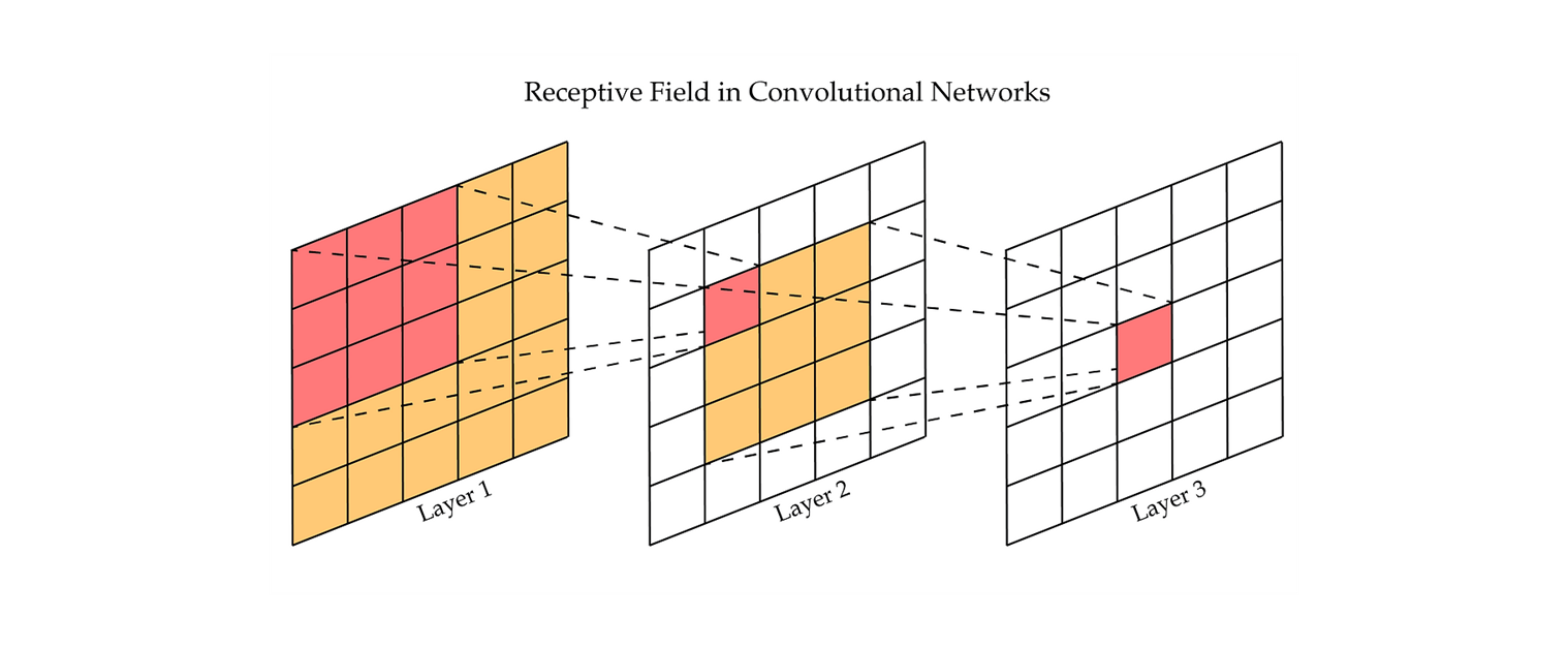
일반적으로 CNN 에서의 Receptive Field 는 image 의 dimension reduction 으로 볼 수 있다.

거기에 kernel 사이즈 안에 들어가 있는 데이터에서 parameter (모수) 를 줄이되, 설명력 있게 특징을 잘 살린 object (개체) 를 뽑아서 나가는 것.

2. Stage

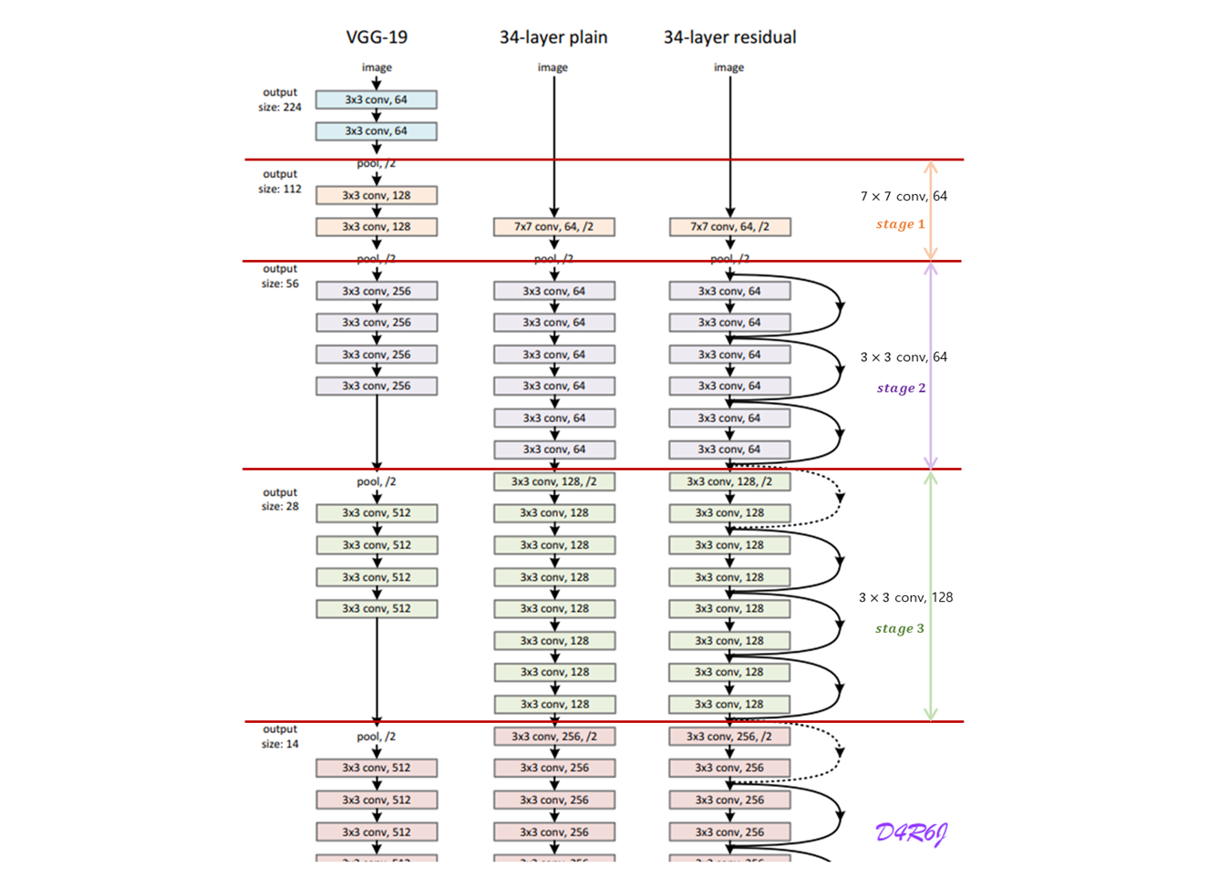
같은 shape 에 같은 filter 를 사용하는 layer 의 구간

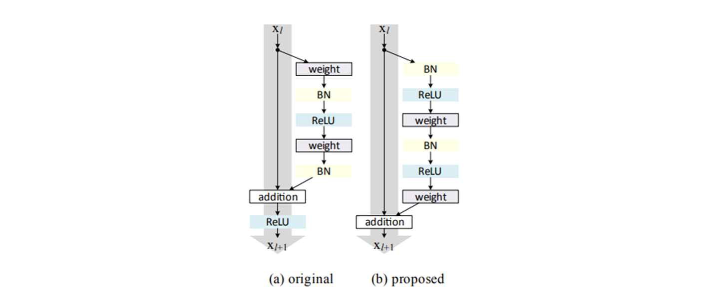
3. identity

Residual Connection 에서 나온 개념, input 정보를 그대로 가지고 있는 개체를 identity.

\mathbf{y} = \mathcal{F}(\mathbf{x}, \{W_i\}) + \mathbf{x}

Various types of shortcut connections.. ( ResNet v2 )

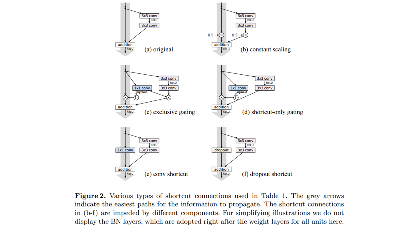
The grey arrows 는 정보를 전파하기 위한 가장 쉬운 길을 나타낸다.
$(b-f)$ 에 있는 shortcut connections 은 다른 components (구성 요소) 에 의해 방해된다.
BN layer 들은 여기 모든 units 에 대한 weight layer 바로 뒤에 채택한다. 그림에선 skip.

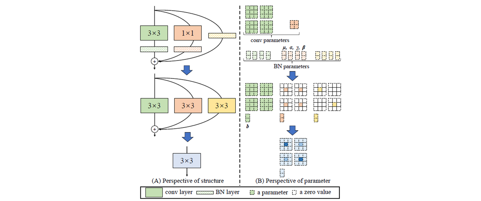
4. RepVGG (Reparameterization VGG)

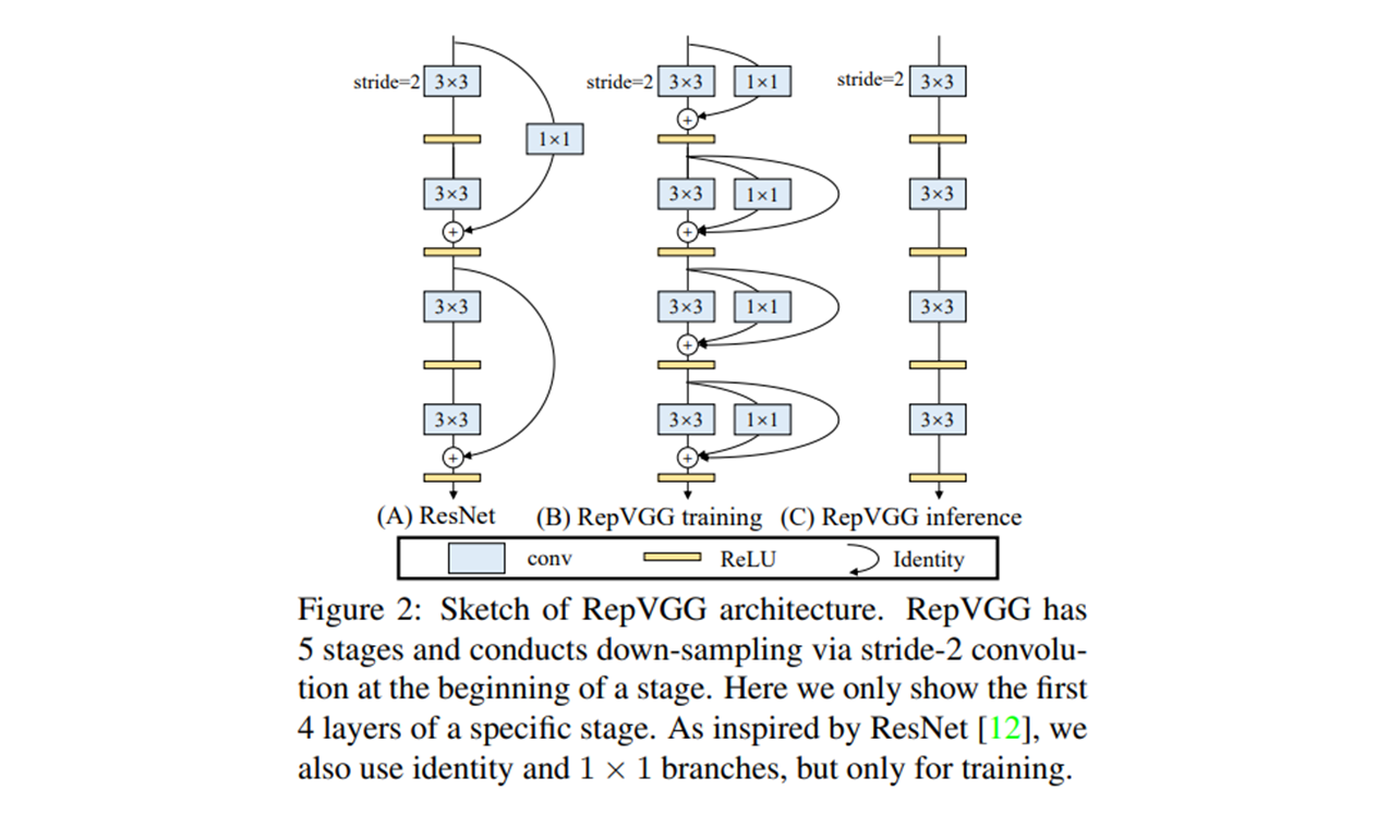
RepVGG 는 5 개의 stage 를 갖고, stage 의 시작에 stride-2 conv 를 사용하여 down-sampling.
identity 와 1x1 conv 는 training 을 위해서 만 사용한다.
training (B) 에 사용한 3x3 conv, 1x1 conv, identity, weight of BN 으로 모델 design 가능.
inference (C) 3x3 conv 만으로 모델 design 가능.

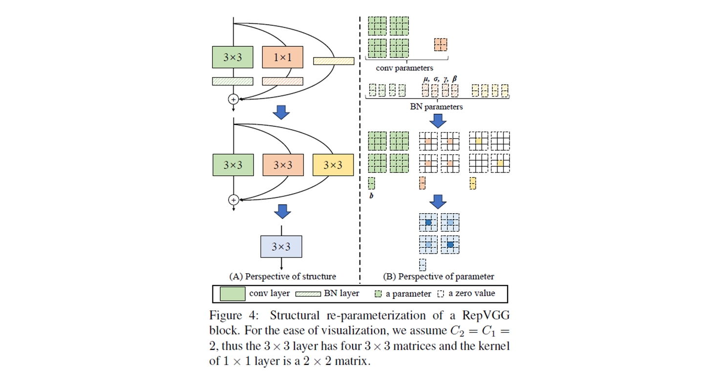
$C_1$ : input channels, $C_2$ : output channels, $C_2 = C_1 = 2$ ,
$3 \times 3$ conv 는 4 개의 $3 \times 3$ matrix 를 갖고, $1 \times 1$ conv 의 kernel 은 $2 \times 2$ matrix 를 갖는다.
# of Input weights : $N \times N \times (I_{nput}) \times (O_{utput})$
- $3 \times 3$ conv $\rightarrow 3 \times 3 \times 2 \times 2 = 36 = (4) \times 3 \times 3 \rightarrow$ $3 \times 3$ conv 4 개.
- $1 \times 1$ conv $\rightarrow 1 \times 1 \times 2 \times 2 = 4 = (4) \times 1 \times 1 \rightarrow 2\times 2$ matrix (4 개).
- BN : hyper parameter $\rightarrow$ $O_{utput} = 2$

여기서 point
1. $1 \times 1$ conv $\rightarrow$ $3 \times 3$ conv
2. identity $\rightarrow$ $3 \times 3$ conv
3. conv + BN $\rightarrow$ conv + bias

Green $3 \times 3$ conv, kernel = 3, stride = 1, padding = 1, BN layer 통과. → $3 \times 3$ conv.
Orange $1 \times 1$ conv, kernel = 1, stride = 1, padding = 1, BN layer 통과..
```
# _pad_1x1_to_3x3_tensor
return torch.nn.functional.pad(kernel1x1, [1,1,1,1])
```
→ zero padding 을 붙여서 $3 \times 3$ conv 로 transformation.
Yellow no conv. input 을 더하고 BN layer 통과.
```
self.rbr_identity = \
	nn.BatchNorm2d(num_features=in_channels) if out_channels == in_channels and stride == 1 else None
```
```
self.se = nn.Identity()
```
identity matrix 로써, 그대로 들어온 matrix 그대로 흘려 보내면 된다. 이것을 $1 \times 1$ conv 로 대체. $1 \times 1$ conv 에 각 channel $C_1 = C_2 = 2$ 이고, 따라서 가중치는
이 되어야 원본. → zero padding 을 붙여서 $3 \times 3$ conv 로 transformation.

$BN$ parameters : $\mu, \sigma, \gamma, \beta \rightarrow \mathbf{b}$
$W$ : weight matrix of kernel
$M$ : Feature map
$C_1$ : input channels
$C_2$ : output channels

\begin{aligned} W^{(3)} &\in \mathbb{R}^{C_2 \times C_1 \times 3 \times 3} : {\rm kernel \; of \; 3 \times 3 \; Conv \; layer} \\ W^{(1)} &\in \mathbb{R}^{C_2 \times C_1} : {\rm kernel \; of \; 1 \times 1 \; branch} \end{aligned}

Accumulated mean, standard deviation and learned scaling factor and bias of $BN$ following $n \times n$ conv
- $\mu^{(n)}, \; \sigma^{(n)}, \; \gamma^{(n)}, \; \beta^{(n)}, \quad {\rm identity \; branch \; is \; } n = 0.$

$M^{(1)} \in \mathbb{R}^{N \times C_1 \times H_1 \times W_1}, \quad M^{(2)} \in \mathbb{R}^{N \times C_2 \times H_2 \times W_2}$
$C_1= C_2, \; H_1 = H_2, \; W_1 = W_2$

\begin{aligned} M^{(2)} &= BN(M^{(1)} * W^{(3)}, \mu^{(3)}, \sigma^{(3)}, \gamma^{(3)}, \beta^{(3)}) \\ & + BN(M^{(1)} * W^{(1)}, \mu^{(1)}, \sigma^{(1)}, \gamma^{(1)}, \beta^{(1)}) \\ & + BN(M^{(1)}, \mu^{(0)}, \sigma^{(0)}, \gamma^{(0)}, \beta^{(0)}) \end{aligned}

$BN$ formula

Conv + BN \rightarrow Conv + bias

y = \gamma \frac{M * W - \mu}{\sqrt{\sigma^2 + \epsilon}} + \beta \approx \gamma \frac{M * W - \mu}{\sigma} + \beta = M * (\frac{\gamma}{\sigma}W) - \gamma \frac{\mu}{\sigma} + \beta

$\epsilon$ 이 매우 작다면, 0 으로 보내고
$W$ 에 $\frac{\gamma}{\sigma}$ 가 곱해지면 새로운 $W'$ 생성
나머지 $\gamma, \mu, \sigma, \beta$ 인 $- \gamma \frac{\mu}{\sigma} + \beta$ 의 조합으로 $\mathbf{b}'$ 생성

M * (\frac{\gamma}{\sigma}W) - \gamma \frac{\mu}{\sigma} + \beta = M * W' + \mathbf{b}'

Here $BN$ is the inference-time $BN$ function, formally, $\forall 1 \leq i \leq C_2,$

BN(M, \mu, \sigma, \gamma, \beta)_{:, i, :, :} = (M_{:, i, :, :}- \mu_i) \frac{\gamma_{i}}{\sigma_{i}} + \beta_{i}.

We first convert every $BN$ and its preceding conv layer into a conv with a bias vector.

Let $\{W', \mathbf{b}'\}$ be the kernel and bias converted from $\{W, \mu, \sigma, \gamma, \beta\}$ , we have

W'_{i,:,:,:}=\frac{\gamma_i}{\sigma_i}W_{i,:,:,:}, \quad \mathbf{b}'_i = \frac{\mu_i\gamma_i}{\sigma_i} + \beta_i

Then it is easy to verify that $\forall 1 \leq i \leq C_2,$

BN(M*W, \mu, \sigma, \gamma, \beta)_{:,i,:,:} = (M*W')_{:,i,:,:} + \mathbf{b}_i'

Green : $3 \times 3$ conv + BN layer → $3 \times 3$ conv + Bias
Orange : $1 \times 1$ conv + BN layer → $3 \times 3$ conv + Bias
Identity + BN : $1 \times 1$ conv + BN layer → $3 \times 3$ conv + Bias

5. Reparameterization trick (Variational Autoencoder)

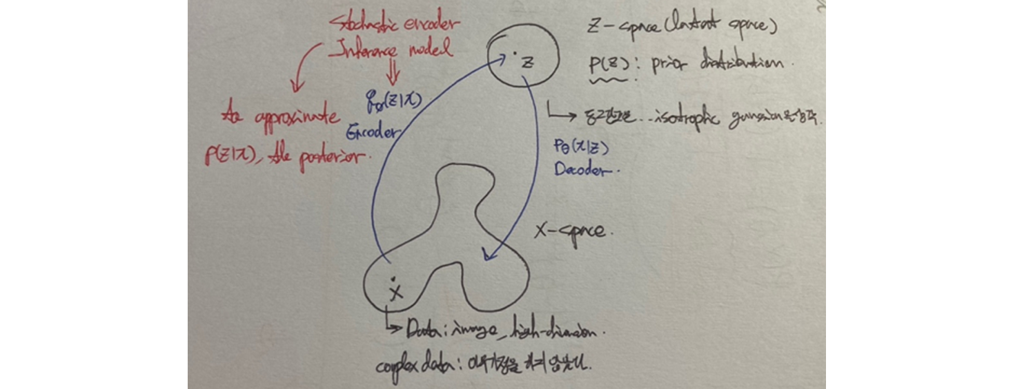
쉽게 이야기하면, Gaussian distribution (random noise) 에서 sampling 을 하는데, one sample approximation ( 생성 ) 하면 한 개의 sample ( constant ) 이므로 미분 불가능하게 되서 $\mu, \sigma$ 를 밖으로 뽑아서 err backpropagation 으로 미분 가능하게 한다는 의미.

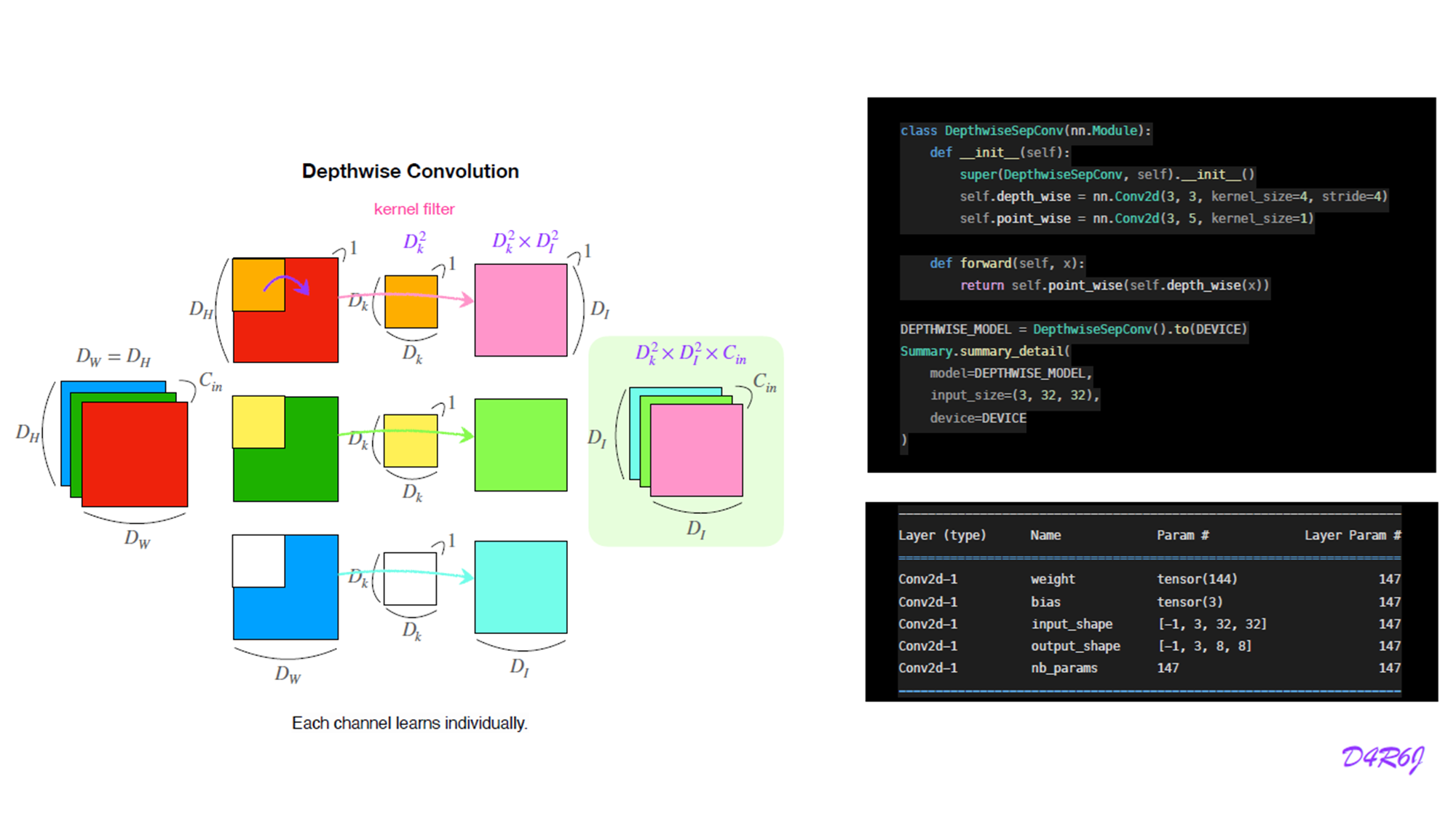
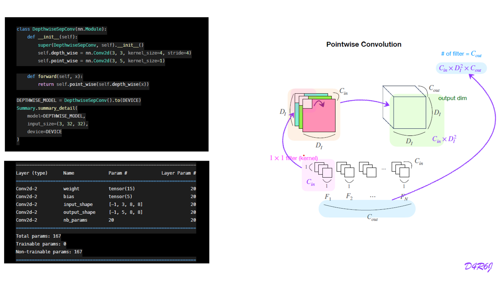
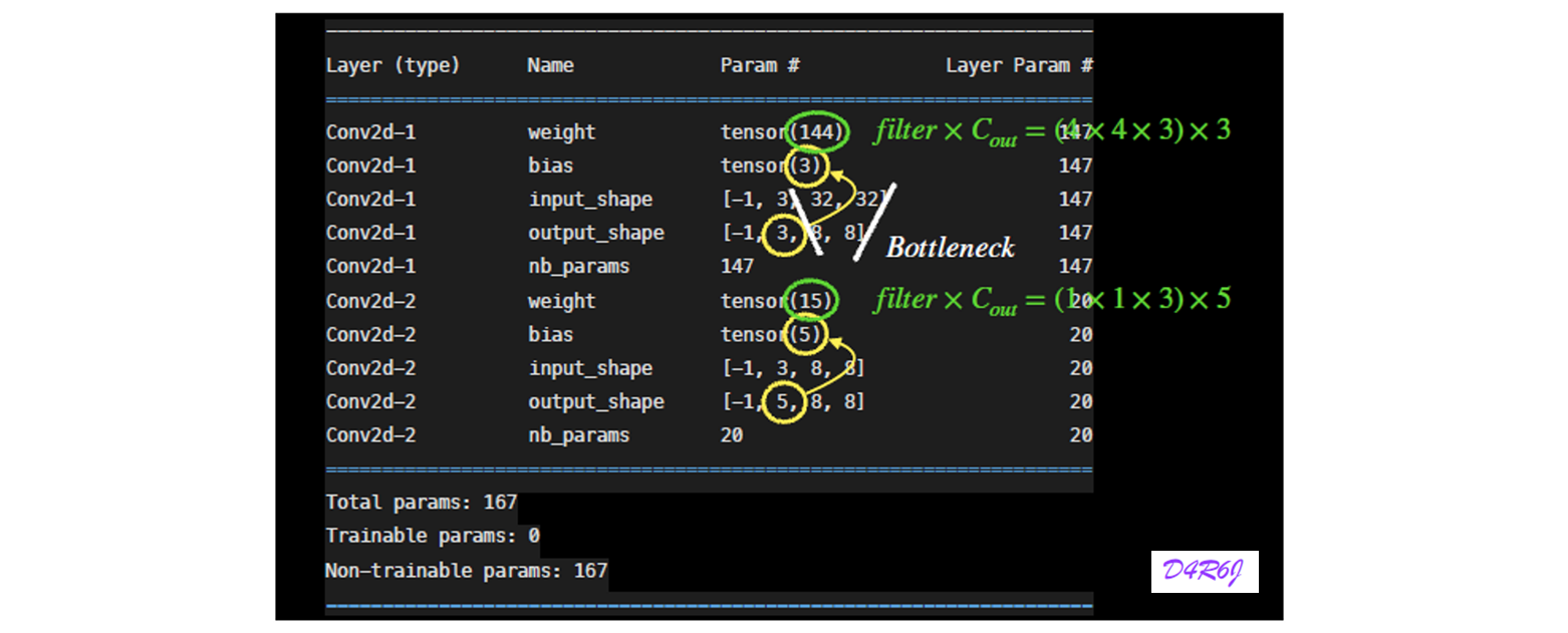
6. Depthwise separable Convolution

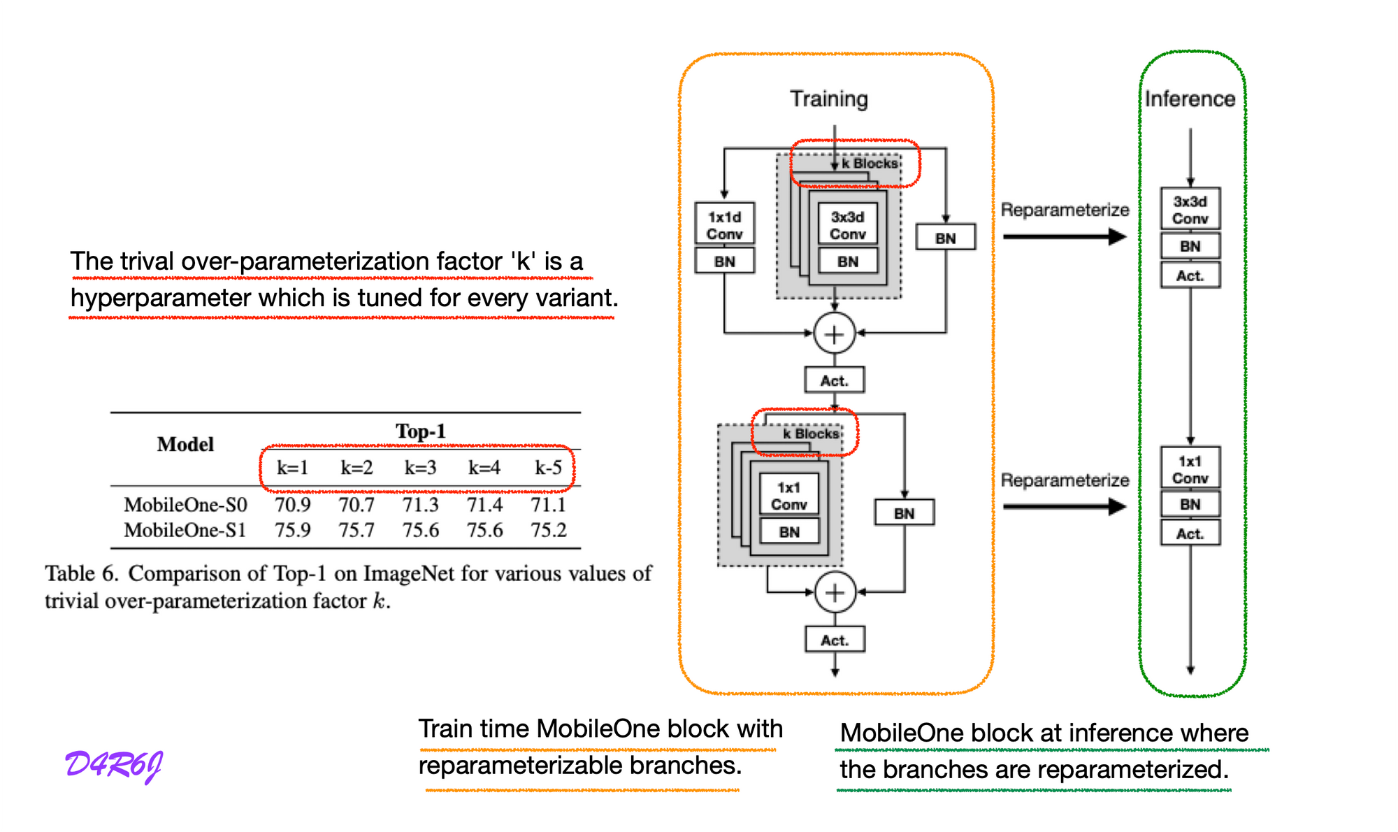
7. MobileOne block

Left : Train time MobileOne block with reparameterizable branches.

 else:
     # Re-parameterizable skip connection
     self.rbr_skip = nn.BatchNorm2d(num_features=in_channels) \
         if out_channels == in_channels and stride == 1 else None

     # Re-parameterizable conv branches
     rbr_conv = list()
     for _ in range(self.num_conv_branches):
         rbr_conv.append(self._conv_bn(kernel_size=kernel_size,
                                       padding=padding))
     self.rbr_conv = nn.ModuleList(rbr_conv)

     # Re-parameterizable scale branch
     self.rbr_scale = None
     if kernel_size > 1:
         self.rbr_scale = self._conv_bn(kernel_size=1,
                                        padding=0)

     # ...
     # Multi-branched train-time forward pass.
   # Skip branch output
   identity_out = 0
   if self.rbr_skip is not None:
       identity_out = self.rbr_skip(x)

   # Scale branch output
   scale_out = 0
   if self.rbr_scale is not None:
       scale_out = self.rbr_scale(x)

   # Other branches
   out = scale_out + identity_out
   for ix in range(self.num_conv_branches):
       out += self.rbr_conv[ix](x)

   return self.activation(self.se(out))

Right : MobileOne block at inference where the branches are reparameterized.

 if inference_mode:
     self.reparam_conv = nn.Conv2d(in_channels=in_channels,
                                   out_channels=out_channels,
                                   kernel_size=kernel_size,
                                   stride=stride,
                                   padding=padding,
                                   dilation=dilation,
                                   groups=groups,
                                   bias=True)
 # ...
 # Inference mode forward pass.
 if self.inference_mode:
     return self.activation(self.se(self.reparam_conv(x)))

Up : depth-wise conv

 # Depthwise conv
 blocks.append(MobileOneBlock(in_channels=self.in_planes,
              out_channels=self.in_planes,
              kernel_size=3,
              stride=stride,
              padding=1,
              groups=self.in_planes,
              inference_mode=self.inference_mode,
              use_se=use_se,
              num_conv_branches=self.num_conv_branches))

Down : point-wise conv

 # Pointwise conv
 blocks.append(MobileOneBlock(in_channels=self.in_planes,
              out_channels=planes,
              kernel_size=1,
              stride=1,
              padding=0,
              groups=1,
              inference_mode=self.inference_mode,
              use_se=use_se,
              num_conv_branches=self.num_conv_branches))

$k$ -Blocks : over-parameterization

 :param num_blocks_per_stage: List of number of blocks per stage.

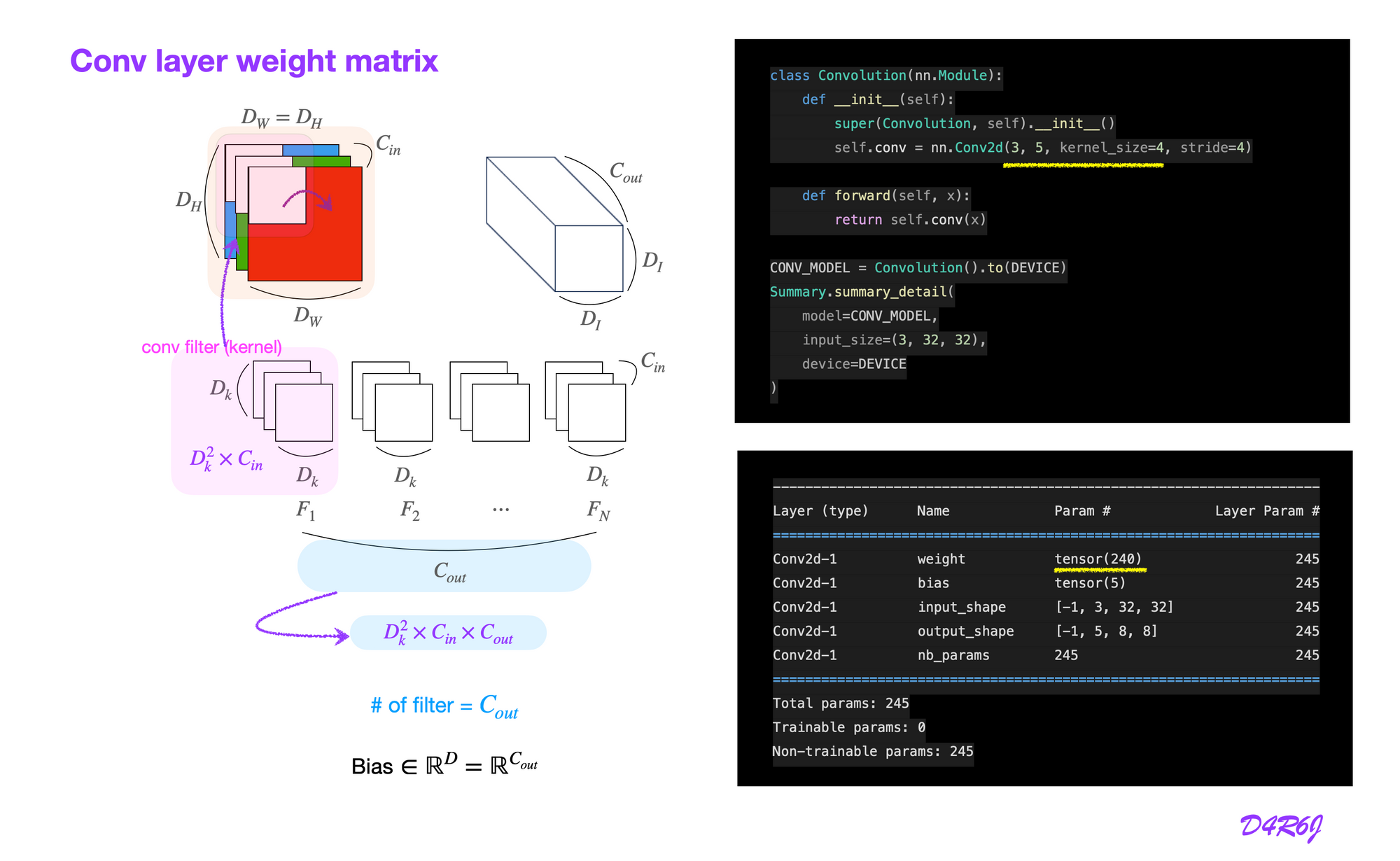
8. Convolution Batch Normalization

Conv layer weight matrix

\mathbf{W'} \in \mathbb{R}^{C_{out} \times C_{in} \times D_K \times D_K}, \; \mathbf{b'} \in \mathbb{R}^D

batch norm layer contains

fuse_bn_tensor

input_dim = self.in_channels // self.groups
kernel_value = torch.zeros(self.in_channels,
							input_dim,
							self.kernel_size,
							self.kernel_size,
							dtype=branch.weight.dtype,
							device=brahch.weight.device)

# padding 1.
for i in range(self.in_channels):
		kernel_value(i, i % input_dim,
					  self.kernel_size // 2,
					  self.kernel_size // 2] = 1

self.id_tensor = kernel_value

	Sequential	else
kernel	branch.conv.weight	self.id_tensor = kernel_value

$\mu$ : accumulated mean
$\sigma$ : accumulated standard deviation
$\gamma$ : scale, $\beta$ : bias

\hat{W} = W' * \frac{\gamma}{\sigma}

gamma = branch.(bn.)weight
std = (running_var + eps).sqrt()
t = (gamma / std).reshape(-1, 1, 1, 1)
return kernel * t

\hat{\mathbf{b}} = (\mathbf{b}' - \mu) * \frac{\gamma}{\sigma} + \beta.

gamma = branch.(bn.)weight
beta = branch.(bn.)bias
std = (running_var + eps).sqrt()
return beta - running_mean * gamma / std

For skip connection the $BN$ is folded to a convolutional layer with identity $1 \times 1$ kernel, which is then padded by $K-1$ zeros as described in RepVGG.

def _get_kernel_bias(self) -> Tuple[torch.Tensor, torch.Tensor]:
    # get weights and bias of scale branch
    kernel_scale = 0
    bias_scale = 0
    if self.rbr_scale is not None:
        kernel_scale, bias_scale = self._fuse_bn_tensor(self.rbr_scale)
        # Pad scale branch kernel to match conv branch kernel size.
        pad = self.kernel_size // 2
        kernel_scale = torch.nn.functional.pad(kernel_scale,
                                               [pad, pad, pad, pad])

\mathbf{W} = \sum^{M}_{i}\hat{W}_i, \quad \mathbf{b} = \sum^{M}_{i}\hat{\mathbf{b}_i}

    # get weights and bias of skip branch
    kernel_identity = 0
    bias_identity = 0
    if self.rbr_skip is not None:
        kernel_identity, bias_identity = self._fuse_bn_tensor(self.rbr_skip)

    # get weights and bias of conv branches
    kernel_conv = 0
    bias_conv = 0
    for ix in range(self.num_conv_branches):
        _kernel, _bias = self._fuse_bn_tensor(self.rbr_conv[ix])
        kernel_conv += _kernel
        bias_conv += _bias

    kernel_final = kernel_conv + kernel_scale + kernel_identity
    bias_final = bias_conv + bias_scale + bias_identity
    return kernel_final, bias_final

for convolution layer at inference is obtained, where $M$ is the number of branches.

def reparameterize(self):

	if self.inference_mode:
	    return

	kernel, bias = self._get_kernel_bias()
	self.reparam_conv = nn.Conv2d(in_channels=self.rbr_conv[0].conv.in_channels,
                            out_channels=self.rbr_conv[0].conv.out_channels,
                            kernel_size=self.rbr_conv[0].conv.kernel_size,
                            stride=self.rbr_conv[0].conv.stride,
                            padding=self.rbr_conv[0].conv.padding,
                            dilation=self.rbr_conv[0].conv.dilation,
                            groups=self.rbr_conv[0].conv.groups,
                            bias=True)
	self.reparam_conv.weight.data = kernel
	self.reparam_conv.bias.data = bias

inference mode

# Delete un-used branches
for para in self.parameters():
    para.detach_()
self.__delattr__('rbr_conv')
self.__delattr__('rbr_scale')
if hasattr(self, 'rbr_skip'):
    self.__delattr__('rbr_skip')

self.inference_mode = True

9. Token mixer

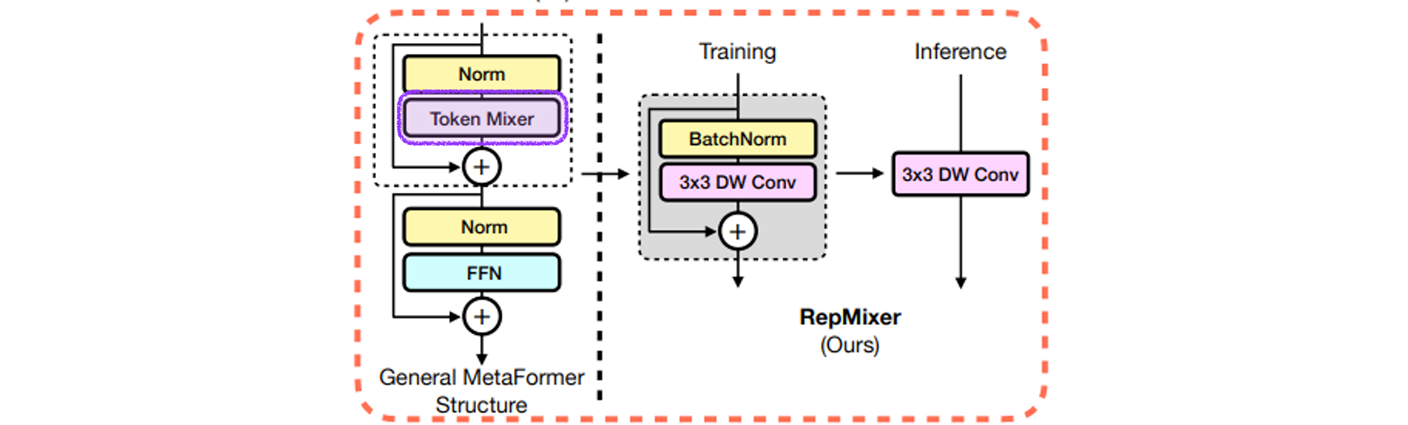
Explain layer
- Transformer = Attention
- MLP-like model = Spatial MLP
- PoolFormer = Pooling
- MetaFormer = Token Mixer ??

transformer 의 성공은 attention-based token mixer 이고, 이것은 다양한 attention 모듈이 ViT 를 항상 시키기 위한 발전을 가져왔다.

그러나 최근 연구에서는 token mixers 로써 spatial MLP 들이 attention 모듈을 교체시 파생된 MLP-like 모델 들이 image classificaion benchmarks 에서 경쟁력 있는 performance 를 낸다.

follow-up works 로는 data-efficient 훈련 과 specific MLP 모듈을 설계하여 ViT 와의 performance gap 을 점차 좁히고, token mixers 로써 attention 의 권위에 도전한다.

@register_model
def metaformer_id_s12(pretrained=False, **kwargs):
   ...
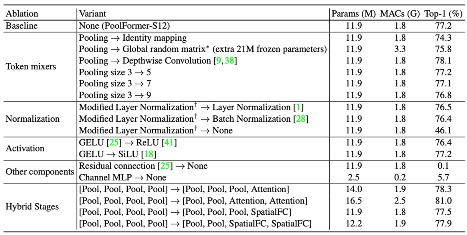
   token_mixers = [nn.Identity] * len(layers)

@register_model
def metaformer_pppa_s12_224(pretrained=False, **kwargs):
   ...
   token_mixers = [Pooling, Pooling, Pooling, Attention]

@register_model
def metaformer_ppaa_s12_224(pretrained=False, **kwargs):
    ...
    token_mixers = [Pooling, Pooling, Attention, Attention]

@register_model
def metaformer_pppf_s12_224(pretrained=False, **kwargs):
    ...
    token_mixers = [Pooling, Pooling, Pooling,
        partial(SpatialFc, spatial_shape=[7, 7]),
    ]

@register_model
def metaformer_ppff_s12_224(pretrained=False, **kwargs):
    ...
    token_mixers = [Pooling, Pooling, 
        partial(SpatialFc, spatial_shape=[14, 14]), 
        partial(SpatialFc, spatial_shape=[7, 7]),
    ]

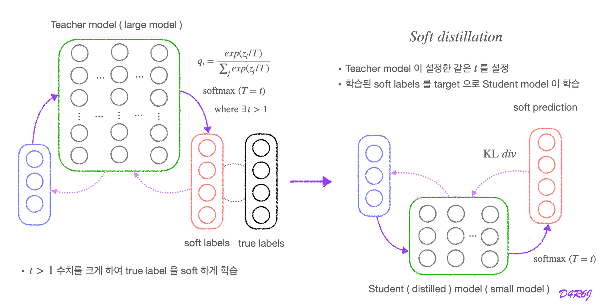
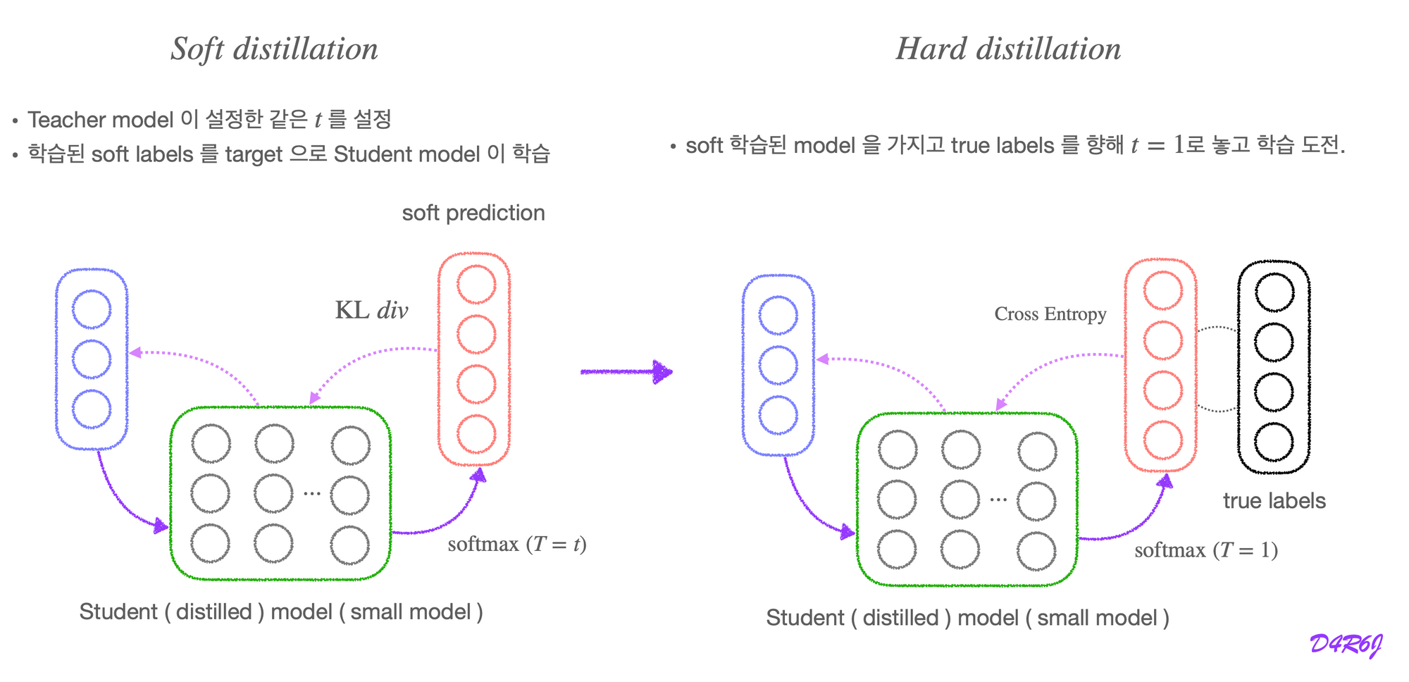
10. Distilling the knowledge in a Neural Network

Review blog https://mr-waguwagu.tistory.com/45

Soft distillation

Hard distillation

Matching logits is a special case of distillation

q_i = \frac{e^{(z_i/T)}}{\sum_{j}e^{(z_j/T)}}

Neural networks typically produce class probabilities by using a “softmax” output layer.

converts the logit $z_i$ ,
computed for each class into a probability $q_i$
$T$ is a temperature that is normally set to $1$ .

logit function is the inverse of the standard logistic function

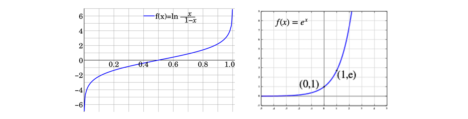
\begin{aligned} \sigma(x) &= \frac{1}{1 + e^{-x}} \\ {\rm logit \;} p = \sigma^{-1}(x) &= {\rm ln \;}\frac{x}{1 - x} \quad {\rm for }\quad p \in (0, 1). \end{aligned}

logit $z_i$ 의 값은 나올 것이고, $T$ 의 값에 따라서 커지면 soft 하고, 작아지면 hard 하게 된다.

Cross-Entropy gradient : $case$ (Hard distillation) with respect to each logit, $z_i$ of the distilled model. If the cumbersome model has logits $v_i$ which produce soft target probabilities $p_i$ and the transfer training is done at a temperature of $T$ ,

\frac{\partial C}{\partial z_i} = \frac{1}{T}(q_i-p_i) = \frac{1}{T} \left( \frac{e^{{z_i}/{T}}}{\sum_{j}e^{z_i/T}} - \frac{e^{{v_i}/{T}}}{\sum_{j}e^{v_i/T}} \right)

If the temperature is high compared with the magnitude of the logits, we can approximate:
$\frac{\partial C}{\partial z_i} \approx \frac{1}{T} \left( \frac{1 + z_i / T}{N + \sum_j z_j/T} - \frac{1 + v_i / T}{N + \sum_j v_j/T}\right)$
If we now assume that the logits have been zero-meaned sparately for each transfer case so that $\sum_jz_j = \sum_jv_j = 0$
$\frac{\partial C}{\partial z_i} \approx \frac{1}{NT^2}(z_i -v_i)$
$T$ 가 작으면 hard 하게 되고, soft 한 정도가 떨어져서 negative logit 들 간 차이가 작아진다.
- soft target 의 distribution function 이 one-hot encoding 에 가까워진다.+
- distilled model 의 negative logit 과의 차이가 더 작아진다.
$T$ 가 크다면 soft 하게 되고, soft 한 정도가 올라가서 negative logit 들 간의 차이가 커진다.
- distilled model 의 negative logit 과의 차이가 더 커진다.
soft target 은 high entropy 라서 일반 학습에 사용하는 hard target 보다 information 이 많다.
training gradient 간의 gradient 의 variance 가 작아서, small model 이 적은 data 로도 효율적으로 학습이 가능해진다.