[ Llama 2 ] analyze model and review code.

d4r6j·2024년 3월 10일

paper-review

nlp-paper

목록 보기

3/8

Llama 2 관련하여 code 와 model architecture 부터 보고, paper 에서 training, tuning 관련 된 내용을 볼 예정이다.

Llama 1 과 관련하여 2 는 차이가 GQA (Groupted Query Attention) 이라는데, 둘다 합하여 못봤던 방법을 정리.

1. RMSNorm

paper : RMSNorm, BatchNorm

Batch Norm

Input: Values of $x$ over a mini-batch: $\mathcal{B} = \{x_{1\cdots m}\};$
Output: $\{y_i = {\rm BN_{\gamma, \beta}(x_i)}\}$

\begin{aligned} \mu_{\mathcal{B}} & \leftarrow \frac{1}{m}\sum^{m}_{i=1}x_i \quad \quad \quad \quad \quad \quad \quad \quad \text{mini-batch mean} \\ \sigma^{2}_{\mathcal{B}} & \leftarrow \frac{1}{m}\sum^{m}_{i=1}(x_i - \mu_{\mathcal{B}})^2 \quad \quad \quad \quad \;\;\; \text{mini-batch variance} \\ \hat{x}_i &\leftarrow \frac{x_i - \mu_{\mathcal{B}}}{\sqrt{\sigma^{2}_{\mathcal{B}}+\epsilon}} \quad \quad \quad \quad \quad \quad\quad \quad\text{normalize} \\ y_i & \leftarrow \gamma \hat{x}_i + \beta \equiv {\rm BN}_{\gamma, \beta}(x_i) \quad \quad \quad \; \text{scale and shift} \end{aligned}

def batch_norm(X, gamma, beta, eps, momentum):
  if len(X.shape) == 2:
    mean = X.mean(dim=0)
    var = ((X - mean) ** 2).mean(dim=0)
  else:
    mean = X.mean(dim=(0, 2, 3), keepdim=True)
    var = ((X - mean) ** 2).mean(dim=(0, 2, 3), keepdim=True)
    
  X_hat = (X - mean) / torch.sqrt(var + eps)
  
  Y = gamma * X_hat + beta
  
  return Y

RMS(Root Mean Square) Norm

\bar{a}_i = \frac{a_i}{RMS(a)}g_i, \quad RMS(a) = \sqrt{\frac{1}{n}\sum^{n}_{i=1}a_i^2}

class RMSNorm(torch.nn.Module):
  def __init__(self, dim: int, eps: float = 1e-6):
      super().__init__()
      self.eps = eps
      self.weight = nn.Parameter(torch.ones(dim))

  def _norm(self, x):
      return x * torch.rsqrt(x.pow(2).mean(-1, keepdim=True) + self.eps)

  def forward(self, x):
      output = self._norm(x.float()).type_as(x)
      return output * self.weight

사용 이유

RMSNorm 은 말 그대로 mean 후 sqrt 만 하는 연산 이라면, BN 은 input (mini-batch) 의 mean, variance 를 구한다.
BN 은 $\gamma, \beta$ 등의 parameter 가 있는 반면, RMSNorm 은 mean 이므로 $n$ 를 나누어 주는 것 말고는 없다.
BN 은 $\gamma \hat{x}_i + \beta$ 선형 변환 이라면, RMS 는 그런 변환이 아니라 일반성이 높다. 직관적으로는 그렇지만, 안정성, 비선형성 에 대한 내용은 좀 더 직접 연구해보고 추가할 예정.

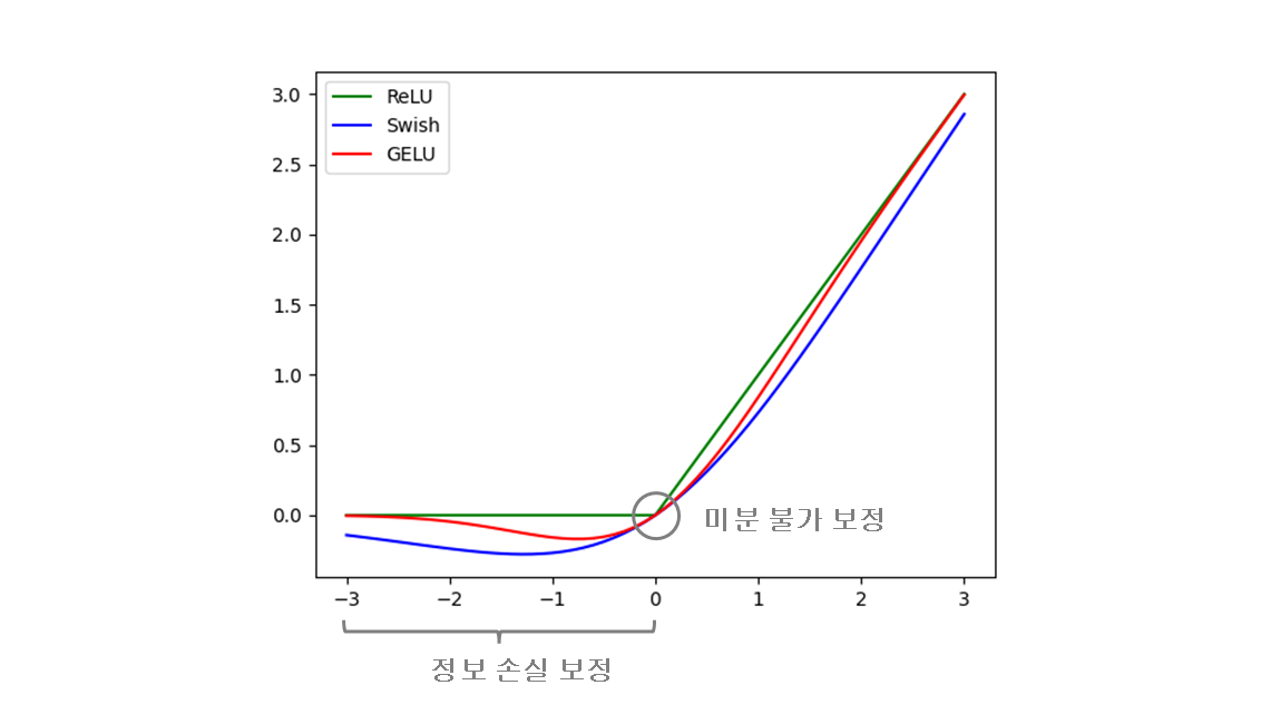
2. SwiGLU

paper : SwiGLU

Swish + GLU (Gated Linear Units)

SILU torch doc

Applies the Sigmoid Linear Unit (SiLU) function, element-wise. The SiLU function is also known as the swish function

{\rm silu}(x) = x * \sigma(x), \quad \text{where } \sigma(x) \text{ is the logistic sigmoid.}

class FeedForward(nn.Module):
    def __init__(
        self,
        dim: int,
        hidden_dim: int,
        multiple_of: int,
        ffn_dim_multiplier: Optional[float],
    ):
        super().__init__()
        hidden_dim = int(2 * hidden_dim / 3)
        # custom dim factor multiplier
        if ffn_dim_multiplier is not None:
            hidden_dim = int(ffn_dim_multiplier * hidden_dim)
        hidden_dim = multiple_of * ((hidden_dim + multiple_of - 1) // multiple_of)

        self.w1 = ColumnParallelLinear(
            dim, hidden_dim, bias=False, gather_output=False, init_method=lambda x: x
        )
        self.w2 = RowParallelLinear(
            hidden_dim, dim, bias=False, input_is_parallel=True, init_method=lambda x: x
        )
        self.w3 = ColumnParallelLinear(
            dim, hidden_dim, bias=False, gather_output=False, init_method=lambda x: x
        )

    def forward(self, x):
        return self.w2(F.silu(self.w1(x)) * self.w3(x))

\begin{aligned} {\rm SwiGLU}(x, W, V, b, c, \beta) &= {\rm Swish}_\beta(xW_1 + b) \otimes (xW_3+c) \\ {\rm FFN}(x, W, V, W_2) &= {\rm SwiGLU}(x, W, V, b, c, \beta)W_2 \end{aligned}

3. Rotary Positional Embeddings (RoPE)

paper : Rotary Positional Embeddings (RoPE)

Positional Embedding 파트는 따로 post 를 하나 만들 예정이다.

Absolute Position Embedding

기존의 Transformer Architecture 를 보면, ( transformer full model )

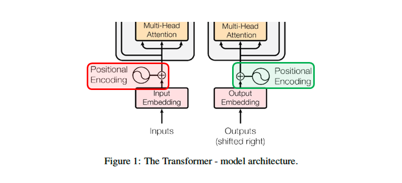
Encoder stack (BERT) 에서는 Input Embedding 다음,
Decoder stack (GPT) 에서는 Output Embedding 다음,
layer 에서 Positional Encoding 을 호출한 것을 볼 수 있다.

이 작업에서 서로 다른 frequencies 의 사인, 코사인 함수를 사용한다.

\begin{aligned} PE_{(pos, 2i)} &= sin(pos/10000^{2i/d_{model}})\\ PE_{(pos, 2i + 1)} &= cos(pos/10000^{2i/d_{model}}) \end{aligned}

transformer PE 로 Absolute Position Embedding 으로, 절대적인 위치 정보를 갖는다.

이러한 경우 extrapolation 에 문제가 된다. 즉, 최대 $N$ 길이로 학습되었다면 $N+1$ 이상의 길이의 position embedding 은 본적이 없게 된다. 그 한계로 inference 시 $N+1$ 이상의 문장이 들어오면 문제가 생긴다.

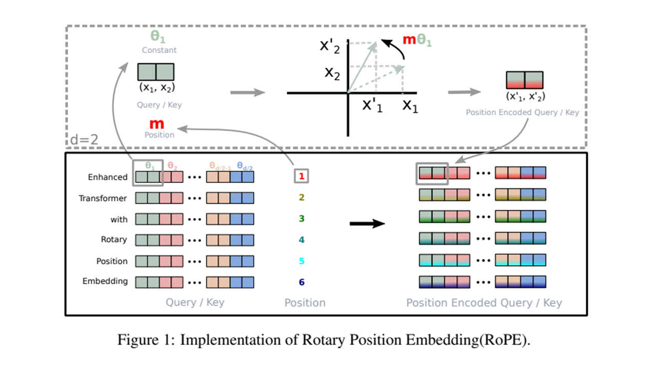
Rotary Positional Embeddings

Relative Position Embedding 중 하나이다. 기존 RPE 는 모두 Additive 형태 이었는데, RoPE 는 Multiplicative + sinusoid 형태 이다. Position Embedding 에 대해서는 따로 post 를 할 예정이다.

query, key : $q, k$
word embeddings : $x_m, x_n$
relative position : $m-n$

query 에서 $m$ 위치의 $x_m$ 단어 임베딩과 key 에서 $n$ 위치의 $x_n$ 단어 임베딩의 내적을 $g$ 함수로 변환하자는 뜻. 여기서 $g$ 함수는 단어 임베딩들과 $m-n$ (상대적 위치) 만 가지고 정의하길 원한다.

inner product 가 상대적 위치로만 위치 정보를 encode 하길 원한다.

\langle f_q(x_m, m), f_k(x_n, n)\rangle = g(x_m, x_n, m-n).

$f_q(x_m, m), f_k(x_n, n)$ 함수를 해결하기 위한 equivalent encoding mechanism 을 찾는 것.

A 2D case

2D Plane 의 기하학적 특성을 사용하면
$\begin{aligned} f_q(x_m, m) &= (W_qx_m)^{e^{im\theta}} \\ f_k(x_n, n) &= (W_kx_n)^{e^{in\theta}} \\ g(x_m, x_n, m-n) &= {\rm Re} \left[(W_qx_m)(W_kx_n)^{*}e^{i(m-n)\theta}\right] \end{aligned}$
여기서 ${\rm Re[\cdot]}$ 는 복소수의 실수 파트 (real number) 이고, $(W_kx_n)^*$ 는 $(W_kx_n)$ 의 켤레 복소수를 나타낸다. $\theta \in \mathbb{R}$ 는 $0$ 이 아닌 상수. multiplication matrix 를 더 보면
$f_{\{q,k\}}(x_m, m) = \begin{bmatrix} \cos m\theta & -\sin m\theta \\ \sin m\theta & \cos m\theta \\ \end{bmatrix} \begin{bmatrix} W^{(11)}_{\{q,k\}} & W^{(12)}_{\{q,k\}} \\ W^{(21)}_{\{q,k\}} & W^{(22)}_{\{q,k\}} \\ \end{bmatrix} \begin{bmatrix} x^{(1)}_m \\ x^{(2)}_m \\ \end{bmatrix}$
affine-transformed 단어 임베딩 벡터를 위치 인덱스 의 각도 배수만큼 회전하고 따라서 Rotary Position Embedding 직관을 해석할 수 있다.

즉, 다시 말하면 $f(x) = Wx + b$ 는 affine transformed 인데 앞에
$\begin{bmatrix} \cos m\theta & -\sin m\theta \\ \sin m\theta & \cos m\theta \\ \end{bmatrix}$
이 2D rotate matrix 이므로 회전 변환을 의미한다. 이것이 Rotary Position Embedding 의 아이디어.

General form

이제 일반화를 시켜보자. 2D 의 결과를 $d$ 가 짝수인, 임의의 $x_i \in \mathbb{R}^d$ 로 일반화 하기 위해 $d$ 차원의 공간을 $\frac{d}{2}$ 하위공간으로 나누고, inner product 의 linearity 로 결합하여

f_{\{q, k\}}(x_m, m) = R^{d}_{\Theta, m}W_{\{q, k\}}x_m

여기서

R^{d}_{\Theta, m} = \begin{bmatrix} \cos m\theta_1 & -\sin m\theta_1 & 0 & 0 & \cdots & 0 & 0 \\ \sin m\theta_1 & \cos m\theta_1 & 0 & 0 & \cdots & 0 & 0 \\ 0 & 0 & \cos m\theta_2 & -\sin m\theta_2 & \cdots & 0 & 0 \\ 0 & 0 & \sin m\theta_2 & \cos m\theta_2& \cdots & 0 & 0 \\ \vdots & \vdots & \vdots & \vdots & \ddots & \vdots & \vdots \\ 0 & 0 & 0 & 0 & \cdots & \cos m\theta_{d/2} & -\sin m\theta_{d/2} \\ 0 & 0 & 0 & 0 & \cdots & \sin m\theta_{d/2} & \cos m\theta_{d/2} \end{bmatrix}

사전 정의된 매개변수들 $\Theta =\{\theta_i =- 10000^{-2(i-1)/d}, i \in [1, 2, \cdots, d/2]\}$ 이 있는 rotary matrix (회전 행렬) 이다.

${\rm RoPE}$ 의 도식 그림은

self-attention 에 RoPE 를 적용하면

q_m^{\top}k_n = (R^{d}_{\Theta, m}W_qx_m)^{\top}(R^{d}_{\theta, n}W_kx_n) = x^{\top}W_qR^{d}_{\theta, n-m}W_kx_n

여기서 $R^{d}_{\Theta, n-m} = (R^{d}_{\Theta, m})^{\top}R^{d}_{\Theta, n}$
$R^{d}_{\Theta}$ 는 position 정보를 encoding 하는 과정에서 안정성을 보장하는 orthogonal matrix 이다. 그러나 이와 같은 행렬 곱셈을 직접 곱하여 적용하는 것은 계산상 효율적이지 않다.

일단, RoFormer 를 이 Post 에서 자세히 다룰 것은 아니고, Position Embedding Post 를 따로 만들어서 자세히 다루어볼 예정이다.

( code ) Rotary Positional Embeddings

def reshape_for_broadcast(freqs_cis: torch.Tensor, x: torch.Tensor):
  ndim = x.ndim
  assert 0 <= 1 < ndim
  assert freqs_cis.shape == (x.shape[1], x.shape[-1])
  shape = [d if i == 1 or i == ndim - 1 else 1 for i, d in enumerate(x.shape)]
  return freqs_cis.view(*shape)

def apply_rotary_emb(
    xq: torch.Tensor,
    xk: torch.Tensor,
    freqs_cis: torch.Tensor,
) -> Tuple[torch.Tensor, torch.Tensor]:
    
    xq_ = torch.view_as_complex(xq.float().reshape(*xq.shape[:-1], -1, 2))
    xk_ = torch.view_as_complex(xk.float().reshape(*xk.shape[:-1], -1, 2))
    freqs_cis = reshape_for_broadcast(freqs_cis, xq_)
    xq_out = torch.view_as_real(xq_ * freqs_cis).flatten(3)
    xk_out = torch.view_as_real(xk_ * freqs_cis).flatten(3)
    return xq_out.type_as(xq), xk_out.type_as(xk)

이 code 에서 보면 궁금한 것은 위에서 설명한 rotary matrix 로 회전변환을 하는데, complex number 를 사용하여 구하는 것을 볼 수 있다. 무슨 관계가 있는지 확인해보자.

2D 설명으로 간단히 관계를 해석해보자. $R^{d}_{\Theta}$ 는 orthogonal matrix 라고 하니 1로 맞춘다.

\begin{aligned} R = \begin{bmatrix} \cos \theta & -\sin \theta \\ \sin \theta & \cos \theta \\ \end{bmatrix} = \begin{bmatrix} \cos \theta & 0 \\ 0 & \cos \theta \\ \end{bmatrix} + \begin{bmatrix} 0 & -\sin \theta \\ \sin \theta & 0 \\ \end{bmatrix} &= \cos\theta \begin{bmatrix} 1 & 0 \\ 0 & 1 \\ \end{bmatrix} + \sin\theta \begin{bmatrix} 0 & -1 \\ 1 & 0 \\ \end{bmatrix} \\ \; \\ \begin{bmatrix} 1 & 0 \\ 0 & 1 \\ \end{bmatrix} = I, \quad \begin{bmatrix} 0 & -1 \\ 1 & 0 \\ \end{bmatrix} = X \quad \longrightarrow \quad R &= \cos\theta \cdot [\;I\;] + \sin\theta \cdot [\;X\;] \end{aligned}

\begin{aligned} R &= \cos\theta \cdot [\;I\;] + \sin\theta \cdot [\;X\;] \\ z &= \cos\theta \cdot 1 + \sin\theta \cdot i \end{aligned}

\begin{aligned} I^2 = \begin{bmatrix} 1 & 0 \\ 0 & 1 \\ \end{bmatrix}^2 = \begin{bmatrix} 1 & 0 \\ 0 & 1 \\ \end{bmatrix} \begin{bmatrix} 1 & 0 \\ 0 & 1 \\ \end{bmatrix} &= I, \quad 1^2 = 1 \cdot 1 = 1 \\ \; \\ X^2 = \begin{bmatrix} 0 & -1 \\ 1 & 0 \\ \end{bmatrix}^2 = \begin{bmatrix} 0 & -1 \\ 1 & 0 \\ \end{bmatrix} \begin{bmatrix} 0 & -1 \\ 1 & 0 \\ \end{bmatrix} = \begin{bmatrix} -1 & 0 \\ 0 & -1 \\ \end{bmatrix} &= -I, \quad i^2 = i \cdot i = -1 \end{aligned}

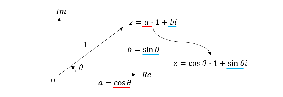
따라서
1. orthogonal rotation matrix 는 unit complex number 와 같다. 이런 intuition 으로 접근
2. rotary positional embedding 에서 as_complex 로 complex number 변환만 나온 이유
3. rotation 이 끝난 후, real part 와 imagenary part 를
4. 다시 as_real 로 돌아가서 기존 dimension 으로 바꾸는 작업을 진행
5. positional embeddings 를 구한다.

( code ) Attention

안에서 query xq 와 key xk 를 가지고 호출한다.


  class Attention(nn.Module):
  # ...
  def forward(
      self,
      x: torch.Tensor,
      start_pos: int,
      freqs_cis: torch.Tensor,
      mask: Optional[torch.Tensor],
  ):
    # ...
    # Rotary Positional Embeddings 에서 확인.
    xq, xk = apply_rotary_emb(xq, xk, freqs_cis=freqs_cis)
    
    self.cache_k = self.cache_k.to(xq)
    self.cache_v = self.cache_v.to(xq)
    
    self.cache_k[:bsz, start_pos : start_pos + seqlen] = xk
    self.cache_v[:bsz, start_pos : start_pos + seqlen] = xv
    
    keys = self.cache_k[:bsz, : start_pos + seqlen]
    values = self.cache_v[:bsz, : start_pos + seqlen]
    
    # repeat k/v heads if n_kv_heads < n_heads
    keys = repeat_kv(keys, self.n_rep)  # (bs, cache_len + seqlen, n_local_heads, head_dim)
    values = repeat_kv(values, self.n_rep)  # (bs, cache_len + seqlen, n_local_heads, head_dim)

Rotary position embedding 을 Attention layer 안에서 한다 apply_rotary_emb. Attention layer 가 여러 개 일때, 각 layer 마다 매번 Position Information 을 Attention 수식에 넣어, 상대적(Relative) Position embedding 을 한다는 뜻.

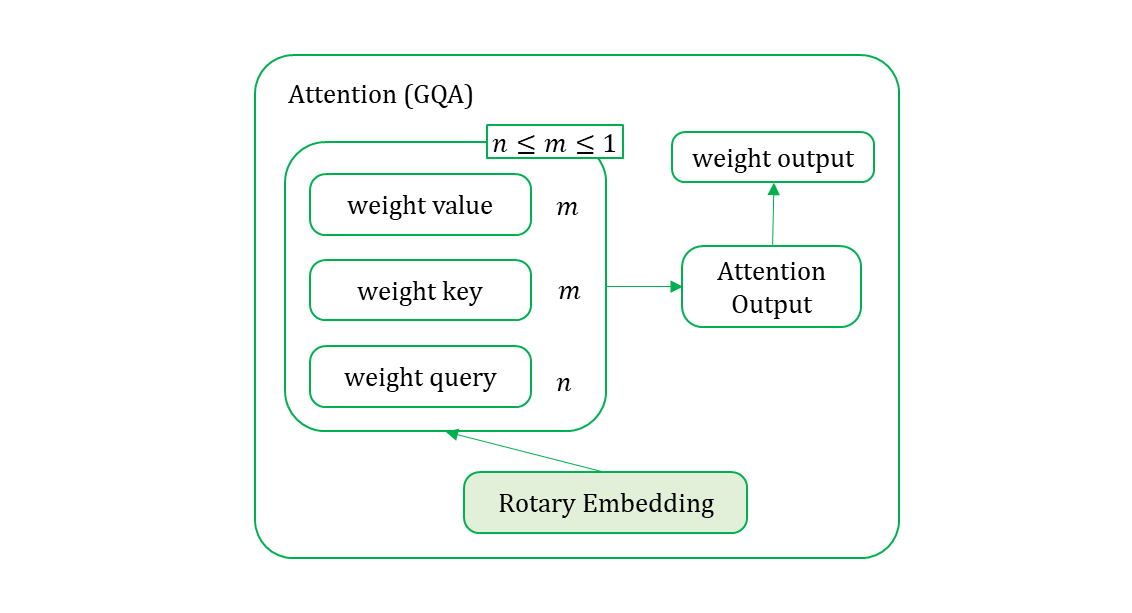
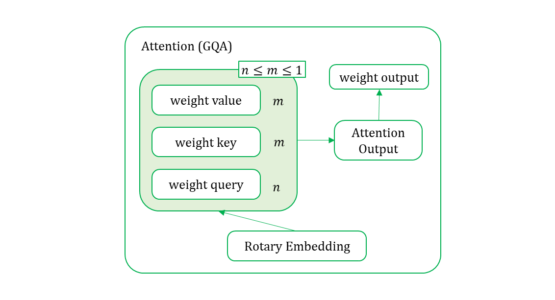
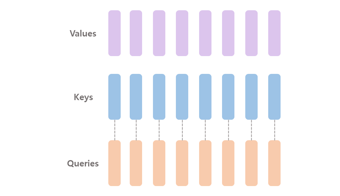
4. Grouped Query Attention (GQA)

paper : Grouped Query Attention (GQA)

Q(uery) K(ey) V(alue)

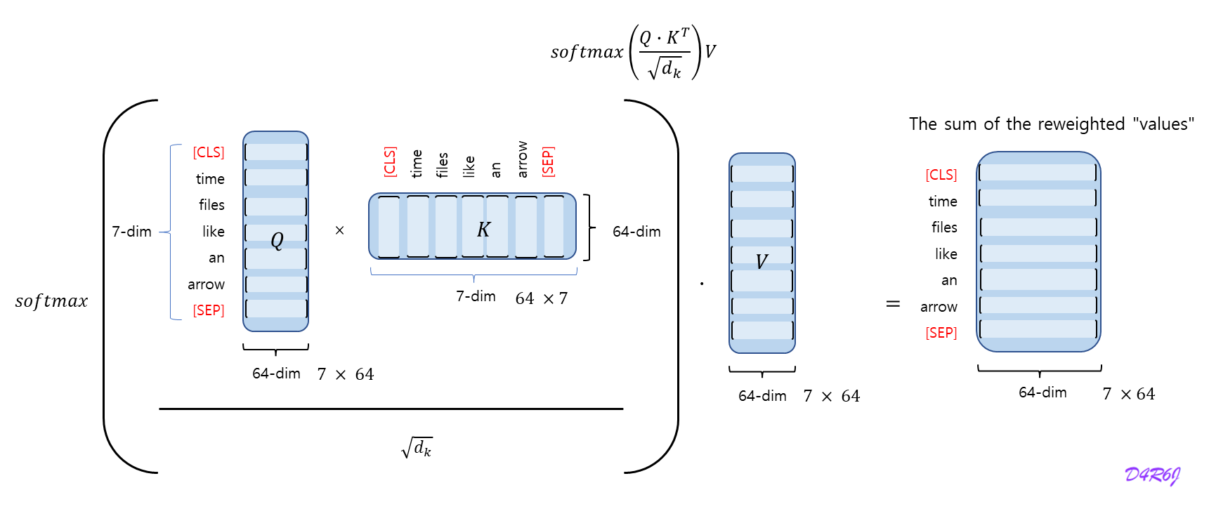
Multi-Head Attention

( code ) Multi-Head Attention

qkv = (
    self.qkv(x)
    .reshape(B, N, 3, self.num_heads, self.num_hidden_dim_head)
    .permute(2, 0, 3, 1, 4)
)
q, k, v = qkv.unbind(0) # make torchscript happy (cannot use tensor as tuple)

# trick here to make q@k.t more stable
attn = (q * self.scale) @ k.transpose(-2, -1)
attn = attn.softmax(dim=-1)
attn = self.attn_drop(attn)

x = (attn @ v).transpose(1, 2).reshape(B, N, C)

Grouped Query Attention

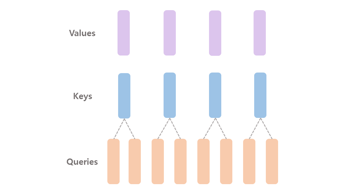
빠르고, 메모리 절약, reduction 이므로 너무 줄이면 정보량 손실이 많으므로 알맞는 값을 찾는것이 중요.

( code ) Grouped Query Attention

GQA 에서 사용할 변수 선언


# n_kv_heads (int): Number of key and value heads.
self.n_kv_heads = args.n_heads if args.n_kv_heads is None else args.n_kv_heads
# n_local_heads (int): Number of local query heads.
self.n_local_heads = args.n_heads // model_parallel_size
# n_local_kv_heads (int): Number of local key and value heads.
self.n_local_kv_heads = self.n_kv_heads // model_parallel_size
self.head_dim = args.dim // args.n_heads

# wq (ColumnParallelLinear): Linear transformation for queries.
self.wq = ColumnParallelLinear(args.dim, args.n_heads * self.head_dim, ...)
# wk (ColumnParallelLinear): Linear transformation for keys.
self.wk = ColumnParallelLinear(args.dim, self.n_kv_heads * self.head_dim, ...)
# wv (ColumnParallelLinear): Linear transformation for values.
self.wv = ColumnParallelLinear(args.dim, self.n_kv_heads * self.head_dim, ...)

self.cache_k = torch.zeros((..., self.n_local_kv_heads, self.head_dim)).cuda()
self.cache_v = torch.zeros((..., self.n_local_kv_heads, self.head_dim)).cuda()

xq, xk, xv = self.wq(x), self.wk(x), self.wv(x)

xq = xq.view(bsz, seqlen, self.n_local_heads, self.head_dim)
xk = xk.view(bsz, seqlen, self.n_local_kv_heads, self.head_dim)
xv = xv.view(bsz, seqlen, self.n_local_kv_heads, self.head_dim)

Query 는 args.n_heads 를 사용하고, Key, Value 는 self.n_kv_heads 를 사용했음을 알 수 있다.
local 은 n_(*)heads 를 model_parallel_size 로 나눈 몫이다.

Attention Algorithm

{\rm softmax}\left( \frac{Q \cdot K^{\top}}{\sqrt{d_k}}\right)V


xq = xq.transpose(1, 2)  # (bs, n_local_heads, seqlen, head_dim)
keys = keys.transpose(1, 2) # (bs, n_local_heads, cache_len + seqlen, head_dim)
values = values.transpose(1, 2) # (bs, n_local_heads, cache_len + seqlen, head_dim)
scores = torch.matmul(xq, keys.transpose(2, 3)) / math.sqrt(self.head_dim)

if mask is not None:
    scores = scores + mask  # (bs, n_local_heads, seqlen, cache_len + seqlen)
scores = F.softmax(scores.float(), dim=-1).type_as(xq)
output = torch.matmul(scores, values)  # (bs, n_local_heads, seqlen, head_dim)

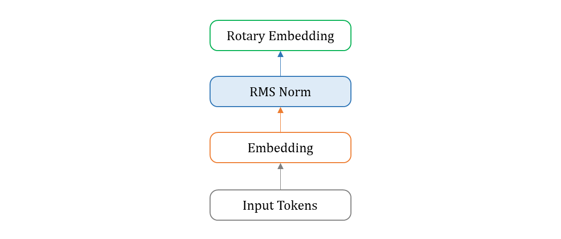
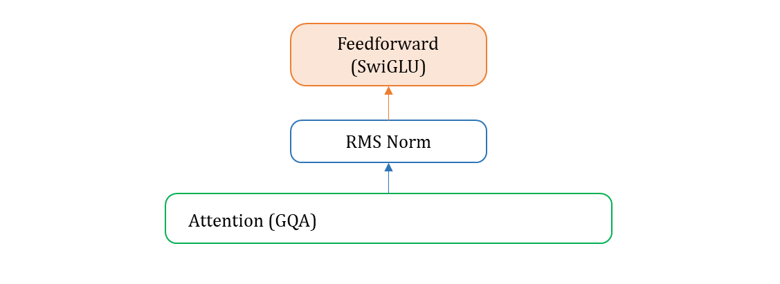
5. Full model

Transformer Block

class TransformerBlock(nn.Module):
    def __init__(self, layer_id: int, args: ModelArgs):
		# ...
        self.attention = Attention(args)
        self.feed_forward = FeedForward(
            # ...
        )
        self.attention_norm = RMSNorm(args.dim, eps=args.norm_eps)
        self.ffn_norm = RMSNorm(args.dim, eps=args.norm_eps)

    def forward(
        self,
        x: torch.Tensor,
        start_pos: int,
        freqs_cis: torch.Tensor,
        mask: Optional[torch.Tensor],
    ):
        h = x + self.attention.forward(
            self.attention_norm(x), start_pos, freqs_cis, mask
        )
        out = h + self.feed_forward.forward(self.ffn_norm(h))
        return out

Transformer

class Transformer(nn.Module):
    def __init__(self, params: ModelArgs):
		# ...
        self.vocab_size = params.vocab_size
        self.tok_embeddings = ParallelEmbedding(
            # ...
        )

        self.layers = torch.nn.ModuleList()
        for layer_id in range(params.n_layers):
            self.layers.append(TransformerBlock(layer_id, params))

        self.norm = RMSNorm(params.dim, eps=params.norm_eps)
        self.output = ColumnParallelLinear(
            params.dim, params.vocab_size, bias=False, init_method=lambda x: x
        )

        self.freqs_cis = precompute_freqs_cis(
            self.params.dim // self.params.n_heads, self.params.max_seq_len * 2
        )

    @torch.inference_mode()
    def forward(self, tokens: torch.Tensor, start_pos: int):
    
        _bsz, seqlen = tokens.shape
        h = self.tok_embeddings(tokens)
        self.freqs_cis = self.freqs_cis.to(h.device)
        freqs_cis = self.freqs_cis[start_pos : start_pos + seqlen]

        # mask logic..
        for layer in self.layers:
            h = layer(h, start_pos, freqs_cis, mask)
        h = self.norm(h)
        output = self.output(h).float()
        return output

하늘색 block 이 TrnasformerBlock 으로 구성. attention_norm 으로 시작, feed_forward 로 block 마무리.
self.output = ColumnParallelLinear 으로 Transformer 의 마지막이 linear 로 구성.

Ref.

Activation function (SwiGLU)
https://medium.com/@tariqanwarph/activation-function-and-glu-variants-for-transformer-models-a4fcbe85323f
GQA (Grouped Query Attention)
https://devocean.sk.com/blog/techBoardDetail.do?ID=165192&boardType=techBlog
Llama2 전반적인 모델 설명
https://velog.io/@alstjsdlr0321/Chapter-8.-LLaMA-2-Part1
Full model 그림 참조.
https://beeny-ds.tistory.com/entry/LLAMA-%EB%AA%A8%EB%8D%B8-%EA%B5%AC%EC%A1%B0-%ED%8C%8C%EC%95%85

d4r6j

이전 포스트

[ Transformer ] paper, code review

다음 포스트