[2021] Deformable DETR

Seong Woong Kim·2022년 11월 9일

Paper Review

목록 보기

1/7

Conference : ICLR (International Conference on Learning Representations)

Authors : Xizhou Zhu, Weijie Su, Lewei Lu, Bin Li, Xiaogang Wang, Jifeng Dai

Published Year : 2021

What is Deformable DETR?

1. 제안 배경

DETR은 Transformer의 Encoder-Decoder 구조를 따서 설계되었습니다.
그리고 many hand-designed components(post-processing : Anchor Generation, Rule-based Training Target Assignment, Non-Maximum Suppression) in object detection을 제거하기 위해 이분 매칭(Bipartite Matching)을 통해 Set Prediction Problem을 직접적으로(directly) 정의해서 해결하려 했습니다.
DETR은 더불어 최초의 fully end-to-end object detector로 소개되었습니다.

하지만, DETR은 Transformer의 특성상 slow convergence와 limitation of Transformer Attention modules in processing image feature maps으로 인한 limited feature spatial resolution으로 어려움을 겪고 있습니다.

이러한 이슈를 해결하기 위해서, Attention modules이 only attend to a small set of key sampling points around a reference하는 Deformable DETR을 제안했습니다.

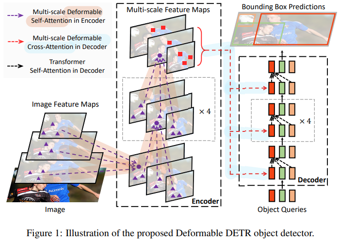
Deformable DETR은 Deformable Convolution으로부터 영감을 받았고, DETR의 구조와 많이 비슷하지만, multi-scale과 DETR에서 사용하는 Transformer의 Attention 방식이 아니라 논문에서 제안된 Multi-Scale Deformable Attention 방식을 도입해서 사용합니다.

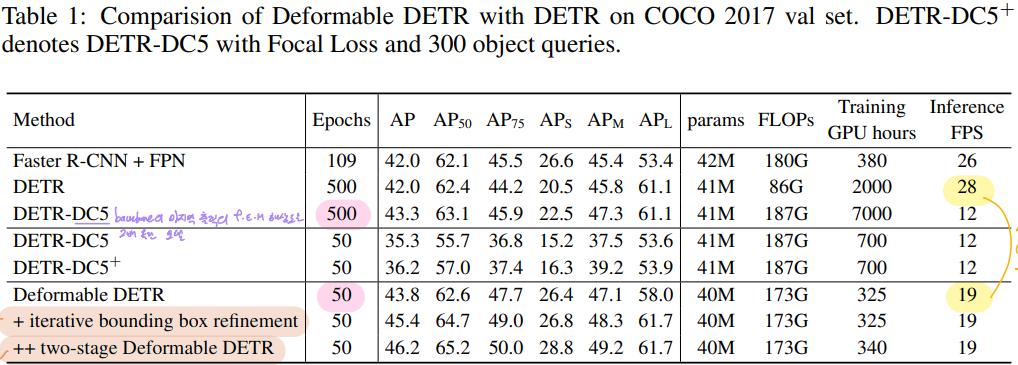
Deformable DETR은 DETR보다 작은 객체들에 대해 더 좋은 성능을 보였고, 10x less training epochs를 사용하였습니다.

1-1. DETR의 두 가지 이슈들

DETR은 Transformer 특성상 크게 2가지 한계점을 가지고 있습니다.

Slow Convergence

모델이 최적으로 수렴하기 위해서 기존 Object Detectors보다 매우 많은 Training epochs가 요구됩니다.

👉 극복하기 위해 Deformable Attention 제안됨

1. Sparse한 Attention이 아닌 Attention Mechanism이라고 하면 모든 input에 대해서 Attention 연산을 수행합니다.

Query가 주어졌을 때, Key 값은 포함된 이미지의 모든 다른 픽셀들이 되는데 이렇게 되는 경우 DETR에서도 학습시간이 굉장히 오래 걸리게 됩니다.

2. Attention이 Object Detection에서는 Attention Weight가 한 곳에 굉장히 포커싱을 해야 하는데, 처음에 Attention이 Uniform한 분포로 돼있기 때문에 포커싱을 하기까지가 굉장히 오랜 시간이 걸립니다.

전형적으로, 파라미터 초기화에서, $U_m$ (input query projection matrix at $m^{th}$ head) $z_q$ (input feature of $q^{th}$ query) and $V_m$ (input key projection matrix at $m^{th}$ head) $x_k$ (input feature of $k^{th}$ key)는 평균 0 & 분산 1인 분포 (uniform)를 따릅니다.

이것은 $N_k$ (number of key elements)이 클 때, attention weight ( $A_{mqk}$ : attention weight of $q^{th}$ query to $k^{th}$ key at $m^{th}$ head)이 key 수만큼 normalization 되는 값과 근사해집니다. ( $\approx \frac{1}{N_k}$ )

이것은 input features에 대해 애매모호한 gradients를 야기하므로 attention weights가 특정한 keys에 포커싱하기 위해서는 긴 훈련 시간을 필요로 하게 됩니다.

이미지 분야에서는 Key elements가 보통 이미지 픽셀로부터 오는데, 픽셀이 엄청 많으므로, 수렴이 엄청 길어집니다.

Low Performance at small objects

DETR은 상대적으로 Small objects를 detect하는데 낮은 성능을 보여줍니다.

극복하기 위해 Multi-scale Deformable Attention 제안됨

1. High-resolution feature maps은 DETR에게 감당할 수 없는 복잡도를 일으킵니다.

현대 Object Detectors는 High-resolution feature maps로부터 작은 객체들이 detect되는 multi-scale features를 사용합니다.
하지만 high-resolution feature maps은 DETR의 Transformer Encoder에 있는 Self-attention momdule에게 Unaccpetable Complexity를 가져다 줍니다.
- 왜냐하면 이 module은 Input feature maps의 공간적인 크기 (픽셀 개수)에 따라 이차원적인(quadratic) 복잡도 증가를 가지기 때문입니다.
  The attention weights computation in the Transformer encoder is of quadratic computation w.r.t. pixel numbers.
  - high-resolution feature maps를 처리하기 위해서 매우 높은 연산량과 메모리 복잡성을 가집니다.
  - 그래서 limitation of Transformer Attention modules in processing image feature maps으로 인한 limited feature spatial resolution으로 어려움을 겪고 있습니다.

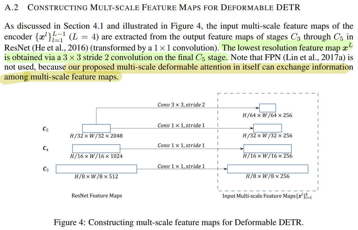
2. Single-Scale Feature Map from ResNet

DETR의 같은 경우 ResNet을 태워서 얻게 되는 feature map의 마지막 feature map을 사용합니다.
마지막 feature map 같은 경우, 작고 정교한 feature는 부족한 feature maps이라고 할 수 있습니다.
이러한 특성 때문에 작은 물체에 대한 탐지 능력이 떨어지게 됩니다. (논문에서는 FPN같은 걸 사용하면 이러한 한계점을 극복한다고 합니다.)
그래서 Deforamble DETR은 FPN은 아니지만 Multi-scale을 이용하게 됩니다.

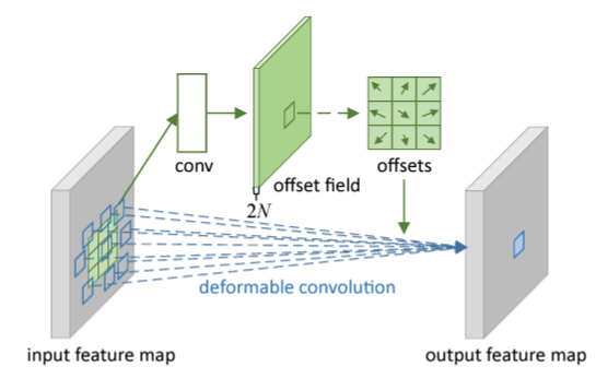
2. Deformable Convolution

Deformable DETR은 Deformable Convlution Networks으로부터 영감을 얻었습니다.

일반적인 Convolution 연산은 고정된 크기의 kernel을 기반으로 수행되지만 deformable convolution은 feature를 특정 layer에 통과시켜 Sampling point를 예측한 후, 해당 point를 기반으로 convolution 연산을 수행합니다.

이미지 분야에서 Deformable Convolution Networks는 Sparse한 공간적인 위치에 접근하는데 매우 강력하고 효과적인 매커니즘입니다.

아래 이미지 예시와 같이 특정 위치의 object들에 맞추어 sampling이 이루어지면서 고정된 크기의 kernel로부터 오는 한계점을 극복하는 것을 확인할 수 있습니다.

일반적인 CNN은 이미지의 물체가 아무리 크더라도 고정된 크기의 필터를 사용하기 때문에 Receptive Field가 커진다는 특성을 이용할 수 있지만, 큰 물체에 대한 탐지 성능이 떨어지는 한계가 있습니다.

이 문제를 극복하기 위해 Deformable Convolution Networks가 제안되었습니다.

Deformable DETR의 경우 매우 비슷한 방법론이라고 할 수 있습니다.

Kernel에 적용하는 게 아니고 Attention Mechanism을 적용할 때 이 Deformable Convolution Networks이란 방법론을 추가해서 적용합니다.

3. Multi-scale Deformable Attention

DETR의 경우 한 스케일 정보에 대해서만 global attention 연산을 수행합니다.

논문에서 제안된 multi-scale deformable attention module은 feature pyramid networks 도움 없이 attention mechanism을 통해서 자연스럽게 multi-scale feature maps을 종합할 수 있다고 합니다. (FPN 효과)

Deformable DETR는 processing feature maps하는 Transformer attention modules를 대체하기 위해서 multi-scale deformable attention modules를 이용합니다.

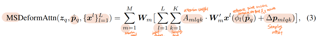
제안된 multi-scale deformable attention module은

자연스럽게 multi-scale feature maps으로 확장이 됩니다.

FPN과 같은 역할을 합니다.

Feature Extraction 단계에서 ResNet에서 32,16,8 같은( $L$ : Level에 비례) 다양한 해상도의 feature maps을 추출한 다음에 각각의 feature map에서 추출한 sample key에 대하여 deformable attention 연산을 수행하게 됩니다.

각 level에서 얻은 sample keys를 모아서 한꺼번에 attention 연산을 수행하기 때문에 각 layer에 있는 각 키에 대한 attention score의 총합이 1이 됩니다.

따라서 Sampling된 key 사이의 관계뿐만 아니라 여러 레벨의 feature maps들 사이의 관계와 정보를 포착하고 자체적으로 교환하게 됩니다

Deformable Convolution의 영향을 받았지만 다른 점이 있습니다.

Single-scale version (deformable convoution)하고 매우 유사하지만, multi-scale deformable attention module은 single-scale feature maps에서 추출한 지정된 개수의 sampling points( $K)$ 만 활용하는 대신에 지정된 레벨의 개수(깊이)와 지정된 sampling points를 곱한 개수만큼을( $LK)$ Sampling 하는 점이 다릅니다.

다양한 크기의 feature maps과 level에서 나온 sampling points를 취합해서 FPN과 같은 효과를 냅니다.

4. Deformable Attention

Transformer Attention을 image feature maps에 적용할 때 큰 이슈는 모든 가능한 위치 정보에 접근한다는 것입니다.

이 문제를 해결하기 위해 Deformable Attention module이 제안됐습니다.
오직 small fixed number of keys for each query에만 attention을 할당함으로써 Convergence Issue와 Feature spatial resolution issue가 완화되었습니다.

Deformable Attention은 Attention 연산을 수행할 때 Key가 모든 픽셀이 되는 것이 아니라, 특정 layer를 통해 예측된 Sampling points들에 대해서만 Attention 연산을 수행합니다. (=Deformable Convolution)

Deformable Attention Module은

모든 픽셀들에 대한 attention을 수행하는 대신, 독립적인 linear layer에 통과시켜 Sampling offset, attention weights를 얻게 되며 이들을 이용하여 attention 연산을 수행하게 됩니다.

이 때 일반적인 방식처럼 내적을 통해 구한 attention weight가 아닌 linear layer를 통해 구한 attention weight를 이용

해당 attention weight를 앞서 구한 sampled points의 feature와 aggregate하여 attention value를 얻습니다.

$A_{mqk}=1$

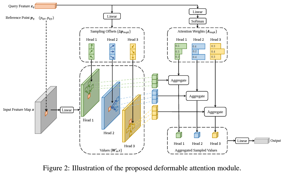
모든 key에 대한 Attention score는 1이기 때문에 일반적인 attention module의 경우 각 key에 부여되는 스코어가 학습 초기에 굉장히 작았으나, deformable attention을 이용하여 특정 개수의 key만 샘플링을 해서, 각 키에 부여되는 score가 충분히 큰 값을 갖게 되었습니다.

deformable attention module은 convolution feature maps을 key elements로써 processing하려고 디자인되었습니다.

5 Loss

Deformable DETR의 Loss는 DETR과 상당히 유사합니다.

5-1. Bipartite Matching (feat. Hungarian Algorithm)

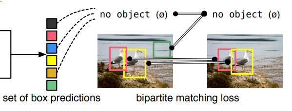
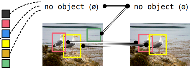
우리의 Loss는 multiple-object 관점에서 ground-truth와 prediction 간의 이상적인 bipartite matching을 생성하고, 그 후 object 단위에서의 loss를 최적화합니다.

< 논문 中 >

Direct Set prediction에서 중요한 두 가지 요소는

예측과 ground truth 사이에 중복이 없는 일대일 매칭을 가능하게 해야 하며,
한 번의 추론에서 object set을 예측하고 그들의 관계를 모델링할 수 있어야 합니다.

👉 이를 만족시키는 object detector를 학습시키기 위해 DETR은 Hungarian Algorithm을 활용한 Bipartite Matching을 통해 loss를 정의합니다.

Object query마다 예측된 결과물 (1 : Class 유무 / 2 : 박스 좌표)과 ground truth set 간 Hungarian algorithm 기반 매칭 수행을 합니다.

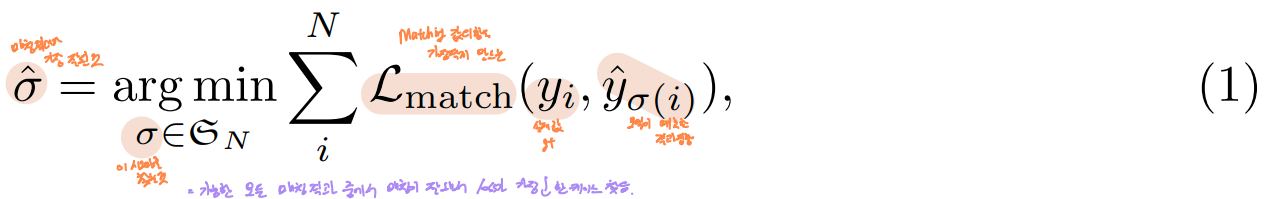
이 때, 매칭의 기준으로 pair-wise matching cost인 $L_{match}$ 를 활용하며, $L_{match}$ 를 최소화하는 최적의 순열( $\hat \sigma$ )을 찾습니다.

이는 Anchor의 비교 방식과 유사하나, anchor는 동일한 ground truth object와의 중복 예측을 허용하는 반면 DETR은 set prediction과 ground truth 간 일대일 매칭을 수행하여 중복을 배제합니다.

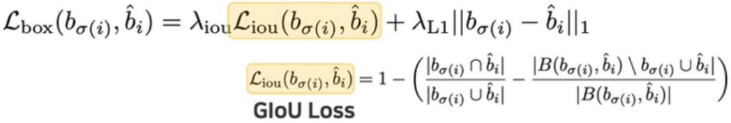
제안된 loss는 이분 매칭 과정을 통한 bounding box 예측에 최적화 되어 있습니다.

즉, $L_{match}(y_i,\hat y _{\sigma(i)})$ 를 ground truth $y_i$ 와 index $\sigma(i)$ 를 갖는 prediction $\hat y _{\sigma(i)}$ 사이의 pair-wise matching cost라 할 때, 위와 같은 permuation을 찾을 수 있게 됩니다

Matching cost는 Class Prediction과 Predicted <> Ground Truth 간 Similarity 두 가지 모두를 고려합니다.

ground truth set의 각 요소 $i$ 관점에서 살펴보면, $c_i$ 를 $Target ~class~ label$ 이라고 하고, $b_i∈[0,1]^4$ 를 ground truth box의 중심 좌표와 높이, 너비에 해당하는 좌표라고 할 때, $y_i=(c_i,b_i)$ 처럼 나타낼 수 있습니다.

또한, 인덱스 $\sigma(i)$ 에 대한 예측을 위해 Class $c_i$ 의 예측확률을 $\hat P \sigma(i)(c_i)$ 라 정의하고, prediction box를 $\hat b_{\sigma(i)}$ 로 정의합니다.

위와 같이 노테이션을 줬을 때, Matching Cost $L_{match}(y_i,\hat y_{\sigma(i)})$ 를 아래와 같이 정의할 수 있습니다.

$\hat P_{\sigma(i)}(c_i)$

순열 $\sigma$ 의 $i$ 번째 요소가 해당하는 Ground Truth의 클래스를 예측한 확률

Class가 일치하면 값이 내려갑니다.

$L_{box}(b_i,\hat b_{\sigma(i)}$

순열 $\sigma$ 의 $i$ 번째 요소의 예측 박스 좌표와 해당하는 Ground Truth의 박스 좌표 간 Loss

Bounding box가 유사하면 값이 올라갑니다.

이 두 가지를 기준으로 Matching을 합니다.

이렇게 Matching을 찾는 과정은 사실 Modern Detector인 proposal(RPN)이나 anchors(FPN)를 ground truth objects에 매칭하는 heuristic assignment rules과 같은 역할을 합니다.

이런 과정은 다른 detector와 다르게 중복되는 prediction이 나오지 않습니다.
다른 점은 duplicates가 없는 direct set prediction을 위한 1-1 매칭을 찾아야 한다는 점입니다.

5-2. Hungarian Loss

Hungrian Loss는 이분 그래프에서 모든 정점에 대한 potential의 합이고, 어떤 할당이 최선의 할당인가?로 모든 쌍을 매칭합니다.

앞선 Hungarian algorithm으로 찾은 '최적의 예측 순열 $\hat \sigma$ 를 이용해 학습을 위한 loss를 계산합니다.

match를 수행하고, match가 된 상황에서 BackPropagation을 위한 Gradient를 흘려주기 위한 Loss 계산합니다.
class prediction과 box의 loss를 위해 negative log-likelihood의 linear combination을 사용합니다.

이 때, $\hat \sigma$ 는 위에서 계산한 Optimal assignment입니다.

설정된 slot의 개수(N=100)에 비해 object의 개수가 훨씬 적으므로(평균 7개) 예측 클래스= $ϕ$ 인 경우가 훨씬 많습니다. (Imbalanced)

이를 해결하기 위해 Faster RCNN의 학습 과정에서 positive/negative proposals의 밸런스를 맞추는 Subsamplilng과 유사한 효과를 위해서 Class = $ϕ$ 일 때, 가중치를 10배 감소시킵니다. (Class = $ϕ$ 일 때의 log-probability term을 factor 10 정도로 down-weight)

$-log\hat P_{\hat \sigma(i)}(C_i)$

Box Loss와의 균형을 위해 Bipartite Matching과 달리 Log Term을 사용합니다.

Class가 유사하도록 만들어줍니다.

Object와 ϕ 사이의 cost는 상수입니다. (Prediction에 의존 X)

이 상황에선 log-probabilities 대신 $\hat P_{\hat \sigma(i)}(C_i)$ 를 대신 사용하여 Class prediction term을 $L_{box}(.)와 상응하게 만들어줍니다.

$L_{box}(b_i,\hat b_{\hat \sigma}(i))$

Box 예측을 합니다.

Class가 ϕ가 아니라면 boudning box또한 잘 맞도록 학습을 시킵니다.

즉, 이분 매칭을 수행해서 어떤 object가 매칭이 됐다고 하면, 실제로 그 매칭 결과가 유사하도록 만들어지기 위해서 매칭된 것들이 각각 다 class 실제 값과 일치하도록 만들고, bounding box또한 유사하도록 만들어줍니다.

5-3. Bounding Box Loss

일반적인 detector에서의 bounding box loss는 예측과 ground truth 간의 상대적인 좌표 및 크기를 이용하여 정의합니다.

(e.g. Anchor에서 정의된 box를 얼마나 움직이고, 얼마나 키워야 ground truth에 가까워지는가)

반면 DETR의 경우, 절대적인 bounding box의 좌표 및 크기를 direct하게 예측하므로 큰 물체와 작은 물체 loss를 계산 시 일반적인 L1 Loss 외에 scale 보정이 필요합니다.
👉 GIoU(Generalized Intersection over Union) 사용

흔히 쓰이는 L1 Loss는 box를 예측할 때 relative error (큰 box와 작은 box의 오차)가 비슷하더라도 small box와 large box 간 다른 scale을 가집니다.

이를 해결하기 위해 (즉, scale-invariant를 보장하기 위해) linear combination of the L1 Loss and generalized IoU Loss를 사용하여 scale을 다양하지 않게 만들어서 이런 문제를 완화시키려 했습니다.

손실 함수로 IoU Loss를 사용하는 이유는 DETR이 작은 객체 검출에 대한 성능이 부족하기 때문에 이를 보완하기 위해서입니다.

IoU 값은 작은 객체든 큰 객체든 면적이 겹치는 비율에 따라 결정되기 때문에, IoU loss를 이용하면 작은 객체도 손실 함수에 크게 기여할 수 있게 됩니다.

이 두 가지 loss는 batch 내부의 object 개수로 normalize합니다.

손실 함수는 각 이미지가 포함하는 객체의 개수에 독립적인 값이어야 하기 때문에, 항상 마지막에 객체 개수로 나눠주어 normalize 하였습니다.

6 Variants for Deformable DETR

논문의 저자들은 Additional Technique를 적용하여 추가적인 성능 향상을 시도했습니다.

Each decoder layer refines the bounding boxes based on the predictions from the previous layer.

$d$ -th decoder layer의 cross attention module에서

그 previous layer( $d^{-1}th$ )의 예측된 bounding box가 $d$ -th new reference point로써 작용합니다.
Sampling offset $\Delta P_{mlqk}$ 도 이전 layer의 예측된 bounding box size에 맞게 조절됩니다.
이러한 수정은 현재 sampling locations이 이전 layer에서 예측된 boxes의 center와 size와 관련이 있게 만듭니다.

6-2. Two-Stage Deformable DETR

Two-stage object detectors에서 영감을 받아서, first stage에서 region proposals을 생성하는 Deformable DETR 변형을 제안했습니다.

First Stage에서 high-recall proposals을 얻기 위해서 multi-scale feature maps에 있는 각 픽셀은 object query로써 작동을 합니다.
decoder를 제거하고, region proposal 생성을 위해 encoder만 있는 Deformable DETR을 만들었습니다.
- 왜냐하면, 직접적으로 object queries를 pixel로 세팅하는 게 감당할 수 없는 연산량과 메모리 cost를 decoder의 self-attention modules 에 가져다주기 때문이다. (self-attention modules은 queries 개수에 따라서 이차원적으로 complexity가 증가하게 됩니다.)
- encoder만 있는 Deformable DETR에서 each pixel은 직접적으로 bounding box를 예측하는 object queries로써 할당이 됩니다.
- 가장 높은 점수를 가진 bounding boxes가 region proposals로써 할당이 됩니다.
- region propsals를 second stage로 반영하기 전에 NMS는 적용되지 않습니다.
- Second stage에서 these region proposals(from the first stage) are fed into the decoder as initial boxes for the iterative bounding box refinement, where the positional embeddings of object queries are set as positional embeddings of region proposal coordinates.

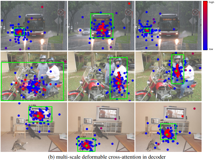
7. Visualization

DETR과 비슷하게, Instance들이 이미 Deformable DETR의 Encoder에서 각각 분리되어 있습니다.

반면에 Decoder에선, DETR이 객체의 오직 extreme points에 집중하는 것에 비해, Deformable DETR은 whole foreground instance에도 집중합니다.

we can guess the reason is that DEformable DETR needs not only extreme points but also interior points to determine object category

DETR은 Encoder에서만 물체를 전반적으로 파악하고 Decoder에서는 물체의 말단 부분에 집중했다면, Deformable DETR은 decoder 단에서도 물체의 내부에 집중하므로 더 탐지 성능이 향상되지 않았나 싶습니다.

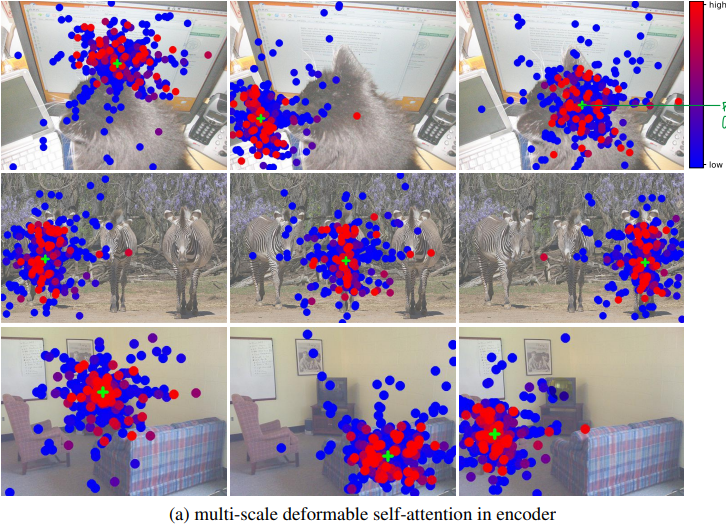
7-1. Multi-scale deformable self-attention in ENCODER

Encoder의 경우 특정 픽셀이 속하는 물체 위주로 (+ : reference point, query point in Encoder) sampling points가 형성되며 형태에 따라 attention weights를 부여하고 있습니다.

7-2. Multi-scale deformable cross-attention in DECODER

Decoder의 경우 물체의 극단 부분에 attention이 몰려 있는 DETR과 다르게 물체의 내부에도 치중된 attention을 주고 있습니다.

Seong Woong Kim

성장과 연구하는 자세를 추구하는 AI 연구개발자

다음 포스트