--08.scikit learn.ipynb--
사이킷런(scikit-learn) 시작
![]()
scikit-learn 특징
- 다양한 머신러닝 알고리즘을 구현한 파이썬 라이브러리
- 심플하고 일관성 있는 API, 유용한 온라인 문서, 풍부한 예제
- 머신러닝을 위한 쉽고 효율적인 개발 라이브러리 제공
- 다양한 머신러닝 관련 알고리즘과 개발을 위한 프레임워크와 API 제공
- 많은 사람들이 사용하며 다양한 환경에서 검증된 라이브러리
scikit-learn의 주요모듈
| 모듈 | 설명 |
|---|---|
sklearn.datasets | 내장된 예제 데이터 세트 |
sklearn.preprocessing | 다양한 데이터 전처리 기능 제공 (변환, 정규화, 스케일링 등) |
sklearn.feature_selection | 특징(feature)를 선택할 수 있는 기능 제공 |
sklearn.feature_extraction | 특징(feature) 추출에 사용 |
sklearn.decomposition | 차원 축소 관련 알고리즘 지원 (PCA, NMF, Truncated SVD 등) |
sklearn.model_selection | 교차 검증을 위해 데이터를 학습/테스트용으로 분리, 최적 파라미터를 추출하는 API 제공 (GridSearch 등) |
sklearn.metrics | 분류, 회귀, 클러스터링, Pairwise에 대한 다양한 성능 측정 방법 제공 (Accuracy, Precision, Recall, ROC-AUC, RMSE 등) |
sklearn.pipeline | 특징 처리 등의 변환과 ML 알고리즘 학습, 예측 등을 묶어서 실행할 수 있는 유틸리티 제공 |
sklearn.linear_model | 선형 회귀, 릿지(Ridge), 라쏘(Lasso), 로지스틱 회귀 등 회귀 관련 알고리즘과 SGD(Stochastic Gradient Descent) 알고리즘 제공 |
sklearn.svm | 서포트 벡터 머신 알고리즘 제공 |
sklearn.neighbors | 최근접 이웃 알고리즘 제공 (k-NN 등) |
sklearn.naive_bayes | 나이브 베이즈 알고리즘 제공 (가우시안 NB, 다항 분포 NB 등) |
sklearn.tree | 의사 결정 트리 알고리즘 제공 |
sklearn.ensemble | 앙상블 알고리즘 제공 (Random Forest, AdaBoost, GradientBoost 등) |
sklearn.cluster | 비지도 클러스터링 알고리즘 제공 (k-Means, 계층형 클러스터링, DBSCAN 등) |
estimator API
- 일관성: 모든 객체는 일관된 문서를 갖춘 제한된 메서드 집합에서 비롯된 공통 인터페이스 공유
- 검사(inspection): 모든 지정된 파라미터 값은 공개 속성으로 노출
- 제한된 객체 계층 구조
- 알고리즘만 파이썬 클래스에 의해 표현
- 데이터 세트는 표준 포맷(NumPy 배열, Pandas DataFrame, Scipy 희소 행렬)으로 표현
- 매개변수명은 표준 파이썬 문자열 사용
- 구성: 많은 머신러닝 작업은 기본 알고리즘의 시퀀스로 나타낼 수 있으며, Scikit-Learn은 가능한 곳이라면 어디서든 이 방식을 사용
- 합리적인 기본값: 모델이 사용자 지정 파라미터를 필요로 할 때 라이브러리가 적절한 기본값을 정의
API 사용 방법
- Scikit-Learn으로부터 적절한
estimator클래스를 임포트해서 모델의 클래스 선택 - 클래스를 원하는 값으로 인스턴스화해서 모델의 하이퍼파라미터 선택
- 데이터를 특징(feature) 배열과 대상(target) 벡터로 배치
- 보통 X, y 로 표현
- 모델 인스턴스의
fit()메서드를 호출해 모델을 데이터에 적합 - 모델을 새 데이터에 대해서 적용
- 지도 학습: 대체로
predict()메서드를 사용해 알려지지 않은 데이터에 대한 레이블 예측 - 비지도 학습: 대체로
transform()이나predict()메서드를 사용해 데이터의 속성을 변환하거나 추론

API 사용하기
import numpy as np
import pandas as pd
import matplotlib.pyplot as plt
import os
plt.style.use(['seaborn-whitegrid']) # 원하는 스타일 지정
x = 10 np.random.rand(50)
y = 2 x + np.random.rand(50)
plt.scatter(x,y)
1. 적절한 estimator 클래스를 임포트해서 모델의 클래스 선택
from sklearn.linear_model import LinearRegression
2. 클래스를 원하는 값으로 인스턴스화해서 모델의 하이퍼파라미터 선택
model = LinearRegression(fit_intercept=True)
model
3. 데이터를 특징(feature) 배열과 대상(target) 벡터로 배치
x
X = x[:, np.newaxis]
X
X[0]
y
4. 모델 인스턴스의 fit() 메서드를 호출해 모델을 데이터에 적합(fit)
model.get_params()
학습(fit)하기 전에는 아래 값들이 없다.
model.coef_ (기울기 값)
model.intercept_ (절편 값)
model.fit(X, y)
모델을 학습한 결과, 학습된 파라미터 들이 있다.
주로 _로 끝나는 값.
model.coef_
model.intercept_
5. 모델을 새 관측 데이터에 적용해본다
xfit = np.linspace(-1, 11)
xfit
Xfit = xfit[:, np.newaxis]
yfit = model.predict(Xfit)
yfit
plt.scatter(x, y) # 학습 데이터
plt.plot(xfit, yfit, '--r') # 예측값
분류(classification) 또는 회귀용(regression) 데이터 세트
| API | 설명 |
|---|---|
datasets.load_boston() | 미국 보스턴의 집에 대한 특징과 가격 데이터 (회귀용) |
datasets.load_breast_cancer() | 위스콘신 유방암 특징들과 악성/음성 레이블 데이터 (분류용) |
datasets.load_diabetes() | 당뇨 데이터 (회귀용) |
datasets.load_digits() | 0에서 9까지 숫자 이미지 픽셀 데이터 (분류용) |
datasets.load_iris() | 붓꽃에 대한 특징을 가진 데이터 (분류용) |
온라인 데이터 세트
- 데이터 크기가 커서 온라인에서 데이터를 다운로드 한 후에 불러오는 예제 데이터 세트
| API | 설명 |
|---|---|
fetch_california_housing() | 캘리포니아 주택 가격 데이터 |
fetch_covtype() | 회귀 분석용 토지 조사 데이터 |
fetch_20newsgroups() | 뉴스 그룹 텍스트 데이터 |
fetch_olivetti_faces() | 얼굴 이미지 데이터 |
fetch_lfw_people() | 얼굴 이미지 데이터 |
fetch_lfw_paris() | 얼굴 이미지 데이터 |
fetch_rcv1() | 로이터 뉴스 말뭉치 데이터 |
fetch_mldata() | ML 웹사이트에서 다운로드 |
예제 데이터 세트 구조
- 일반적으로 딕셔너리 형태로 구성
- data: 특징 데이터 세트
- target: 분류용은 레이블 값, 회귀용은 숫자 결과값 데이터
- target_names: 개별 레이블의 이름 (분류용)
- feature_names: 특징 이름
- DESCR: 데이터 세트에 대한 설명과 각 특징 설명
from sklearn.datasets import load_diabetes
diabetes = load_diabetes() # 결과 dict 형태
diabetes.keys()
data 에는 feature 벡터가 담겨 있다.
diabetes.data
diabetes.target # target값은 수치형! => 이건 '회귀' 문제다!
len(diabetes.data), len(diabetes.target)
print(diabetes.DESCR)
diabetes.feature_names
diabetes.data[0]
model_selection 모듈
- 학습용 데이터와 테스트 데이터로 분리
- 교차 검증 분할 및 평가
- Estimator의 하이퍼 파라미터 튜닝을 위한 다양한 함수와 클래스 제공
학습/테스트 세트 분리
from sklearn.model_selection import train_test_split
X_train, X_test, y_train, y_test = train_test_split(
diabetes.data, diabetes.target, test_size=0.3
)
len(X_train), len(y_train)
len(X_test), len(y_test)
model = LinearRegression()
model.fit(X_train, y_train)
model.score(X_train, y_train)
model.score(X_test, y_test)
점수가 너무 낮다
왜 그런지 시각화를 통해 알아보자
predicted = model.predict(X_test)
expected = y_test
plt.figure(figsize=(8,4))
plt.scatter(expected, predicted)
plt.plot([0, 500], [0,500], '--r')
교차 검증 : cross_val_score()

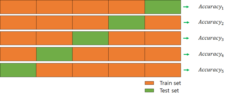
from sklearn.model_selection import cross_val_score, cross_validate
scores = cross_val_score(model, diabetes.data, diabetes.target, cv=5)
cv=5 : 몇등분 할지 (k-fold)
cv 값 개수만큼 score들이 리턴된다.
scores
np.mean(scores), np.std(scores)
GridSearchCV
최적의 하이퍼 파라미터값 찾기
↓GridSearchCV
cross validation 을 여러번 반복해서, 여기에서 최적의 하이퍼 파라미터 를 찾음
그런데 왜? Grid?
Grid ..(촘촘하게) 이리도 돌려보고, 저리도 돌려보며, 최적의 하이퍼 파라미터 를 찾는 것을 GridSearchCV 를 통해서 할수 있습니다.
학습을 통해 최적의 파라미터를 찾는 것은 어려운 일이다. 그래서, 훈련과정을 자동화 하여 cross_validation 검사를 해서
최적값을 제공하는 도구가 필요했는데, GridSearchCV 가 그 역할을 하는 것이다
※ 이하에서 '파라미터' 라 함은 '하이퍼 파라미터' 를 말하는 겁니다.
from sklearn.model_selection import GridSearchCV
from sklearn.linear_model import Ridge # Ridge 모델은 alpha라는 하이퍼 파라미터를 갖고있음.
Ridge().get_params()
GrodSearchCV 할 alpha값들을 7개 정의
alpha= [0.001, 0.01, 0.1, 1, 10, 100, 1000]
GridSearchCV() 의 매개변수로 넘겨줄 parameter값 준비(dict)
param_grid = dict(alpha = alpha)
param_grid
gs = GridSearchCV(estimator = Ridge(), param_grid = param_grid, cv = 10)
각 파라미터 조합마다 cross validatrion x 10번씩 수행\
result = gs.fit(diabetes.data, diabetes.target)
result.bestscore # 최적의 점수
최적 파라미터
result.bestparams
최적 파라미터를 학습된 모델
result.bestestimator
pd.DataFrame(result.cvresults)
cross validation 을 수정한 결화
위 params*** 컬럼을 보면 각 'alpha'값 7개에 대해서 CV돌린 결과를 보여준다.
multiprocessing을 이용한 GridSearchCV
import multiprocessing
from sklearn.datasets import load_iris # 붗꽃 품종 데이터(분류형)
from sklearn.linear_model import LogisticRegression
iris = load_iris()
iris.data
iris.feature_names
iris.target
print(iris.DESCR)
LogisticRegression().get_params()
GridSearchCV 에 넘겨줄 parameter 준비
param_grid = [{
'penalty' : ['l1', 'l2'],
'C' : [0.5, 1.0, 1.5, 1.8, 2.0, 2.4]
}]
multiprocessing.cpu_count()
gs = GridSearchCV(estimator=LogisticRegression(), param_grid=param_grid, cv=10,
scoring='accuracy',
n_jobs = multiprocessing.cpu_count()
)
result = gs.fit(iris.data, iris.target)
result.bestscore
result.bestparams
pd.DataFrame(result.cvresults)
최적점수 : 0.98!1 <-- iris 데이터는 너무 잘된다.!
{'C': 2.4, 'penalty': 'l2'} <-- 최적 파라미터
최적 파라미터값이 우리가 설정한 것의 경계선에 가까우면 , 다시 param_grid 값의 범위를 조정한뒤 돌려보는 것을 추천합니다.
DataFrame 은 C 값 2개 x penalty 값 2개 조합 12개의 행으로 나온다.
위 최적 parameter 로 직접 estimator 생성가능.
LogisticRegression(C=2.4, penalty='l2')
LogisticRegression(**result.bestparams)
preprocessing
데이터 전처리 모듈
scikit-learn 의 preprocessing 모듈
데이터 전처리 는 많은 작업들을 하게 되는데,
대표적인게 scaling 입니다.
데이터의 feature scaling 이라고도 합니다.
scaling 방법은 크게 두가지가 있습니다.
1. 표준화 (standardization)
2. 정규화 (normalization)
정규화와 표준화는 모두 머신러닝 알고리즘을 훈련시키는데 있어서
사용되는 특성(feature)들이 '모두 비슷한 영향력'을 행사하도록
값을 변환해주는 전처리 기술입니다

StandardScaler : 표준화
iris_df = pd.DataFrame(data=iris.data, columns=iris.feature_names)
iris_df
iris_df.describe()
from sklearn.preprocessing import StandardScaler
scaler = StandardScaler()
스케일링을 위해 몇가지 과정을 거쳐야 한다
step 1 : 기본적으로 fit 을 하여 표준화/정규화에 필요한 정보들을 가져옵니다.
step 2 : 가져온 정보에 따라서 scaling 을 위한 transform 메소드를 호출하여
scaling 된 변환을 거칩니다.
위 step1, step2 를 '동시에' 에 수행하는 fit_transform()
iris_scaled = scaler.fit_transform(iris_df) # 스케일링된 결과 리턴(array 형태로.)
iris_scaled.shape
iris_df_scaled = pd.DataFrame(data=iris_scaled, columns = iris.feature_names)
iris_df_scaled
mean은 0
std는 1에 맞추는 스케일링 수행결과
iris_df_scaled.describe()
위 scaling된 데이터로 모델 학습
X_train, X_test, y_train, y_test = \
train_test_split(iris_df_scaled, iris.target, test_size = 0.3)
model = LogisticRegression()
model.fit(X_train, y_train)
훈련 데이터 점수
model.score(X_train, y_train)
테스트 데이터 점수
model.score(X_test, y_test)
정규화 클래스 : MinMaxScaler
from sklearn.preprocessing import MinMaxScaler
scaler = MinMaxScaler()
fit_scaler = scaler.fit(iris_df)
iris_scaled = scaler.transform(iris_df)
iris_df_scaled = pd.DataFrame(data = iris_scaled, columns = iris.feature_names)
iris_df_scaled.describe()
정규화
min 0 , max 1 로 scaling 결과
X_train, X_test, y_train, y_test = \
train_test_split(iris_df_scaled, iris.target, test_size = 0.3)
model = LogisticRegression()
model.fit(X_train, y_train)
print('훈련 데이터 점수 : {}'.format(model.score(X_train, y_train)))
print('평가 데이터 점수 : {}'.format(model.score(X_test, y_test)))
성능평가 지표
metirics 모듈
정확도(Accuracy)
- 정확도는 전체 예측 데이터 건수 중 예측 결과가 동일한 데이터 건수로 계산
- scikit-learn에서는
accuracy_score함수를 제공
from sklearn.datasets import make_classification # 랜덤으로 분류형 데이터 생성
from sklearn.linear_model import LogisticRegression
from sklearn.metrics import accuracy_score
랜덤 분류형 데이터 생성
X, y = make_classification(
n_samples = 1000, # 생성하는 데이터 개수
n_features = 2, # feature의 개수
n_informative = 2, # 의미 있는 feature의 개수
n_redundant=0, # 노이즈 (0 <- 거의 순수한 데이터?)
n_clusters_per_class=1, # 클래스당 하나의 클러스터만 나오게 하기
)
X
y
train, test 구분
X_train, X_test, y_train, y_test = train_test_split(X, y, test_size=0.3, random_state=36)
모델
model = LogisticRegression()
학습
model.fit(X_train, y_train)
model.score(X_train, y_train)
model.score(X_test, y_test)
accuracy 확인하기
predict = model.predict(X_test) # 예측값
accuracy_score(y_test, predict)
오차 행렬(Confusion Matrix)
- True Negative: 예측값을 Negative 값 0으로 예측했고, 실제 값도 Negative 값 0
- False Positive: 예측값을 Positive 값 1로 예측했는데, 실제 값은 Negative 값 0
- False Negative: 예측값을 Negative 값 0으로 예측했는데, 실제 값은 Positive 값 1
- True Positive: 예측값을 Positive 값 1로 예측했고, 실제 값도 Positive 값 1

from sklearn.metrics import confusion_matrix
confmat = confusion_matrix(y_true=y_test, y_pred=predict) # 결과는 2차원 array
print(confmat)
fig, ax = plt.subplots(figsize=(2.5, 2.5))
ax.matshow(confmat, cmap=plt.cm.Blues, alpha=0.3)
for i in range(confmat.shape[0]) :
for j in range(confmat.shape[1]) :
ax.text(x = j, y = i, s=confmat[i,j], va='center', ha='center')
정밀도(Precision)와 재현율(Recall)
-
정밀도(Precision) = TP / (FP + TP)
-
재현율(Recall) = TP / (FN + TP)
-
정확도(accuracy) = (TN + TP) / (TN + FP + FN + TP)
-
오류율 = (FN + FP) / (TN + FP + FN + TP)
from sklearn.metrics import precision_score, recall_score
precision = precision_score(y_test, predict)
precision
recall = recall_score(y_test, predict)
recall
업무 특성에 따라
재현율이 상대적으로 더 중요한 지표인 경우는 실제 Positive 양성인 데이터 예측을 Negative 음성으로 잘못 판단하게 되면 업무상 큰 영향이 발생하는 경우
정밀도가 상대적으로 더 중요한 지표인 경우는 실제 Negative 음성인 데이터 예측을 Positive 양성으로 잘못 판단하게 되면 업무상 큰 영향이 발생하는 경우
재현율이 중요한 경우 -> 암 판단 모델이나 금융 사기 적발 모델과 같이 실제 Positive 양성 데이터를 Negative로 잘못 판단하게 되면 업무상 큰 영향이 발생하는 경우이다.
암 인데(Positive) 암이 아니라고 (Negative) 잘못 판단하면 위험.
정밀도가 중요한 경우 -> 스팸메일 여부를 판단하는 모델과 같은 경우는 정밀도가 더 중요한 지표
스패이아닌데 (Negative) 스팸이라고(Positive) 잘못 판단하면 곤란
재현율이 중요하다 하여 무조건 재현율을 높인다면 무조건 Positive 라 하면 된다.
그러면, 정밀도가 떨어지겠죠.
정밀도와 재현율은 한쪽으로 치우치지 않는게 중요.
F1 Score(F-measure)
- 정밀도와 재현율을 결합한 지표
- 정밀도와 재현율이 어느 한쪽으로 치우치지 않을 때 높은 값을 가짐
\begin{equation}
F1 = 2 \times \frac{precision \times recall}{precision + recall}
\end{equation}
from sklearn.metrics import f1_score
f1_score(y_test, predict)
ROC 곡선과 AUC
-
ROC 곡선은 FPR(False Positive Rate)이 변할 때 TPR(True Positive Rate)이 어떻게 변하는지 나타내는 곡선
- TPR(True Positive Rate): TP / (FN + TP), 재현율
- TNR(True Negative Rate): TN / (FP + TN)
- FPR(False Positive Rate): FP / (FP + TN), 1 - TNR
-
AUC(Area Under Curve) 값은 ROC 곡선 밑에 면적을 구한 값 (1이 가까울수록 좋은 값)
from sklearn.metrics import roc_curve
예측 확률 계산
model.predict_proba(X_test)[:10]
클래스가 1 인것에 대한 확률 값
pred_proba_class1 = model.predict_proba(X_test)[:, 1]
pred_proba_class1[:10]
ROC Curve 를 형성할 수 있는 값들을 리턴해줌.
fprs, tprs, thresholds = roc_curve(y_test, pred_proba_class1)
plt.plot(fprs, tprs, label='ROC') # 매우 좋은 성능을 나타내고 있다.
plt.xlabel('FPR')
plt.ylabel('TPR(Recall)')
plt.legend()
POC Curve 의
아래 영역이 AUC (1에 가까울수록 좋음.)
from sklearn.metrics import roc_auc_score
roc_auc_score(y_test, predict)