3. RL algorithms: Policy-based RL

Recap: Basic of Reinforcement Learning

input
agent, environment

agent take the state($s_t$)
$\rightarrow$ agent take action
$\rightarrow$ action에 따라 환경(state $s_{t+1}$) 변화

objective function
Expected cumulative reward
$R(\tau) = \underset{t=0}{\overset{\infty}{\sum}}\gamma^tr_t\quad\quad$ $where\quad0<\gamma<1$

RL Problem
expected cumulative reward를 최대화 시키는 policy 채택

$\pi$를 policy라고 할 때,
$\pi^* = \underset{\pi}{\mathrm{argmax}}E\big[R(\tau)\big]$

• expected 함수는
  • $s_0$이 주어진 경우, Value function
  • $s_0, a_0$이 주어진 경우, Q function

Taxonomy of RL algorithm

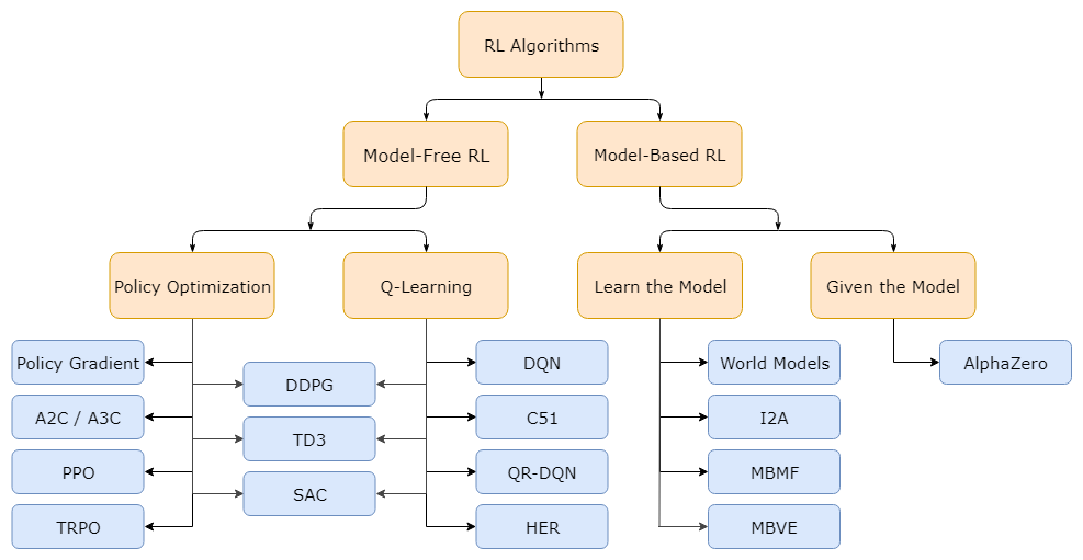
• Model-Free RL : agent는 environment에 대해 아무 정보도 가지고 있지 않음
  대부분의 RL모델들의 기반
  • Policy Optimization : objective function으로 최적화
    RL에서 제일 간단한 편
    • Policy Gradient : objective function을 gradient descent로 optimize하는 모델
  • Q-Learning : Value/Q function으로 학습
• Model-Based RL : agent는 environment의 작동 방식에 대해 알고 있음

일단 이 정도만 알아놓고 가겠음

The goal of Reinforcement Leraning

여기서 policy $\pi_\theta$에 따른 probability distribution over a sequence of trajectory 식을 표현하면

$p_\theta(\tau) = p_\theta(s_1,a_1,...,s_T,a_T)=p(s_1)\underset{t=1}{\overset{T}{\Pi}}\pi_\theta(a_t|s_t)p(s_{t+1}|s_t,a_t)$

식을 풀어보면 이해가 좀 더 잘 되는데...

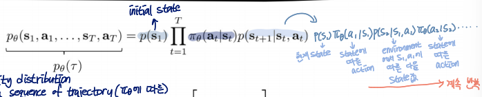
이런 이유로 저렇게 도출됨

Goal of RL

일단 그래서 위의 식을 통한 RL의 goal은
$\theta^* = \underset{\theta}{\mathrm{argmax}}E_{\tau \sim p_\theta(\tau)}\big[\underset{t}{\sum}r(s_t, a_t)\big]$
미분이 어려워서 원래 objective function에서의 discounted factor는 작성 생략됨

정리를 하자면
policy를 따라서 trajectory가 생성되는데, 가장 적절한 trajectory가 포함되어 있는 probability distribution을 만들어내는 policy의 parameter를 찾아내는 것이 목표!

infinite한 경우

$\theta^* = \underset{\theta}{\mathrm{argmax}}E_{(s,a) \sim p_\theta(s,a)}\big[r(s,a)\big]$

finite한 경우(certain timestep에서 끝날 것이라고 가정한 경우)

$\theta^* = \underset{\theta}{\mathrm{argmax}}\underset{t=1}{\overset{T}{\sum}} E_{(s_t,a_t) \sim p_\theta(s_t,a_t)}\big[r(s_t, a_t)\big]$
그냥 아까 식에서 $\sum$이 밖으로 빠지고, T에서 끝난다는 게 생긴 거 말고 다른 거 없음

Evaluating Objective

$\theta^* = \underset{\theta}{\mathrm{argmax}}E_{\tau \sim p_\theta(\tau)}\big[\underset{t}{\sum}r(s_t, a_t)\big]$

$J(\theta) = E_{\tau \sim p_\theta(\tau)}\big[\underset{t}{\sum}r(s_t, a_t)\big] \approx \frac{1}{N} \underset{i}{\overset{N}{\sum}} \underset{t}{\sum} r(s_{i,t}, a_{i,t})$
real world의 policy를 N time 학습했다는 가정
(i,t): i-th sample에서 t번째 timestep
여기서 $\underset{i}{\overset{N}{\sum}}$은 sum over samples from $\pi_\theta$

그런데

• initial probability: $p(s_1)$
• transition probability: $p(s_{t+1}|s_t)$

이 두 값을 모르는데 $J(\theta)$를 어떻게 구하는 걸까?

roleplay를 통해 N번의 sampling을 하고, 이걸 다 더해서 1/N을 취하면 real world의 어느정도는 따라갈 것이라고 가정을 함으로써 해결
그래서 N의 값이 커질수록 estimate가 더 정확해짐
근데 솔직히 내가 잘 이해한 건지 모르겠음..

Direct policy differentiation

$J(\theta) = E_{\tau \sim p_\theta(\tau)}\big[\underset{t}{\sum}r(s_t, a_t)\big] = E_{\tau \sim p_\theta(\tau)} \big[r(\tau)\big]$

$E(x) = \int p(x)dx$

위의 식을 사용해서 식을 바꾸면,
$J(\theta) = \int p_\theta(\tau)r(\tau)d\tau$
여기서 $r(\tau)$는 상수

미분하면,
$\bigtriangledown_\theta J(\theta) = \int\bigtriangledown_\theta p_\theta(\tau)r(\tau)d\tau$

a convenitent identity
$p_\theta(\tau)\bigtriangledown_\theta log p_{\theta}(\tau) = p_\theta (\tau) \frac{\bigtriangledown_\theta p_\theta (\tau)}{p_\theta (\tau)} = \bigtriangledown_\theta p_\theta (\tau)$

위의 식을 사용하면,
$\bigtriangledown_\theta J(\theta) = \int p_\theta (\tau)\bigtriangledown_\theta \log p_\theta(\tau)r(\tau)d\tau = E_{\tau\sim p_\theta (\tau)} \big[\bigtriangledown_\theta \log p_\theta (\tau)r(\tau)\big]$
이렇게 표현이 됨

$p_\theta(\tau) = p_\theta(a_1,a_1,...,s_T,a_T) = p(s_1)\underset{t=1}{\overset{T}{\Pi}}\pi_\theta(a_t|s_t)p(s_{t+1}|s_t,a_t)$
log of both sides
$\log p_\theta(\tau) = \log p(s_1)+\underset{t=1}{\overset{T}{\sum}}\log \pi_\theta(a_t|s_t) + \log p(s_{t+1}|s_t,a_t)$

위를 따르면
$\bigtriangledown_\theta\log p_\theta(\tau)r(\tau) = \bigtriangledown_\theta \big[\log p(s_1)+\underset{t=1}{\overset{T}{\sum}}\log \pi_\theta(a_t|s_t) + \log p(s_{t+1}|s_t,a_t)\big]$

$\log p(s_1)$과 $\log p(s_{t+1}|s_t,a_t)$는 상수($\theta$에 depend하지 않음)이기 때문에 미분 과정 중 0이 됨

따라서,
$\bigtriangledown_\theta J(\theta) = E_{\tau \sim p_\theta(\tau)} \big[(\underset{t=1}{\overset{T}{\sum}}\bigtriangledown_\theta\log \pi_\theta(a_t|s_t))(\underset{t=1}{\overset{T}{\sum}}r(s_t,a_t))\big] = \frac{1}{N} \underset{i=1}{\overset{N}{\sum}}(\underset{t=1}{\overset{T}{\sum}}\log \pi_\theta(a_{i,t}|s_{i,t}))(\underset{t=1}{\overset{T}{\sum}}r(s_{i,t},a_{i,t}))$

이제 다 알려진 value들이라서 계산이 가능해짐!
$\theta \leftarrow \theta + \alpha\bigtriangledown_\theta J(\theta)$

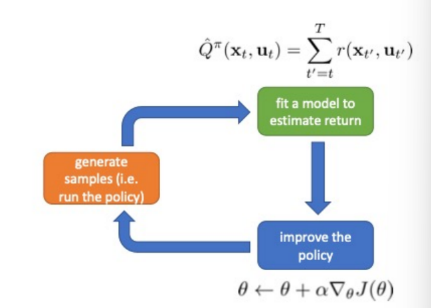
Policy gradient algorithm

1. sample $\{\tau^i\}$ from $\pi_\theta(a_t|s_t)$ (run the policy)
   sample 생성
2. $\bigtriangledown_\theta J(\theta) \approx \underset{i}{\sum}(\underset{t}{\overset{T}{\sum}}\log \pi_\theta(a_{i,t}|s_{i,t}))(\underset{t}{\overset{T}{\sum}}r(s_{i,t},a_{i,t}))$
   fit a model to estimate return
3. $\theta \leftarrow \theta + \alpha\bigtriangledown\theta J(\theta)$
   improve the policy

Comparison to maximum likelihood

policy gradient는 maximum likelihood의 weighted version이라고 볼 수 있음!

• policy gradient
  $\bigtriangledown_\theta J(\theta) \approx \frac{1}{N} \underset{i=1}{\overset{N}{\sum}}(\underset{t=1}{\overset{T}{\sum}}\log \pi_\theta(a_{i,t}|s_{i,t}))(\underset{t=1}{\overset{T}{\sum}}r(s_{i,t},a_{i,t}))$
• maximum likelihood
  $\bigtriangledown_\theta J_{ML}(\theta) \approx \frac{1}{N} \underset{i=1}{\overset{N}{\sum}}(\underset{t=1}{\overset{T}{\sum}}\log \pi_\theta(a_{i,t}|s_{i,t}))$

Example: Gaussian policies

action이 continuous함

• example: $\pi_\theta(a_t|s_t) = N(f_{\text{neural network}}(s_t); \Sigma)$
  action이 continuous하기 때문에 $\mu , \Sigma$ 설정함
• $\log \pi_\theta(a_t|s_t) = -\frac{1}{2}\lVert f(s_t)-a_t \rVert_{\Sigma}^2 + const$
• $\bigtriangledown_\theta\log\pi_\theta(a_t|s_t) = -\frac{1}{2}\Sigma^{-1}(f(s_t)-a_t)\frac{df}{d\theta}$

필요한 값들 구했으니 이제 알고리즘 식에 넣어서 사용하면 됨

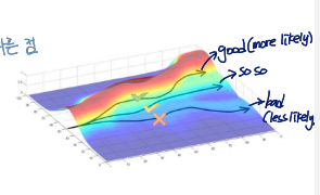
What did we just do?

$\bigtriangledown_\theta J(\theta) \approx \frac{1}{N} \underset{i=1}{\overset{N}{\sum}}(\underset{t=1}{\overset{T}{\sum}}\log \pi_\theta(a_{i,t}|s_{i,t}))(\underset{t=1}{\overset{T}{\sum}}r(s_{i,t},a_{i,t}))$

가중치를 통해 good stuff(trajectory)는 more likey, bad stuff는 less likely하게 만들어짐
trial and error를 통해 더 많은 가중치를 주는 trajectory를 더 자주 선택할 수 있도록 만듦

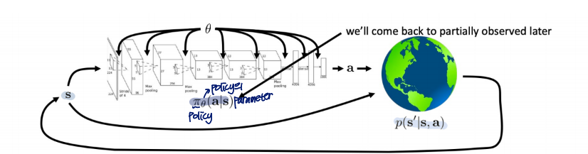
Partial observability

에이전트가 환경의 전체 상태 $s_t$를 직접 관찰할 수 없고, 대신 그 상태에 대한 부분적인 정보인 관찰치(observation) $o_t$만을 받게 되는 경우,

objective function의 형태는 같음
그냥 $\pi_\theta$의 변수에서 state를 observation으로만 바꾸면 됨

$\bigtriangledown_\theta J(\theta) \approx \frac{1}{N} \underset{i=1}{\overset{N}{\sum}}(\underset{t=1}{\overset{T}{\sum}}\log \pi_\theta(a_{i,t}|o_{i,t}))(\underset{t=1}{\overset{T}{\sum}}r(s_{i,t},a_{i,t}))$

Markov property is not actually used!

can use policy gradient in partially observed MDP(Markov Decision Property)'s without modification

Problem of Policy Gradient

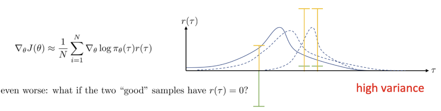
현재 위의 그래프에는 three samples가 있음

• 연두색 : 1차 reward
• 노란색 : 2차 reward

1차 때,
맨 왼쪽의 sample은 large negative reward로 인해 distribution이 오른쪽으로 shift될 것임
negative sample을 less likely하게 만들기 위해

그런데 positive reward를 받는 경우에는 negative reward를 받았을 때보다 조금만 shift되게 됨

high variance의 문제

샘플링의 패턴에 따라 distribution of the policy는 다른 결과를 보임
→ there is a very high variance of the distribution of the policy when we use the policy gradient

Reducing variance

Causality

policy at time $t'$는 본인보다 이전 time의 reward에 영향을 주지 못함
이건 Morkov property와 별개의 개념으로 항상 맞음 (Markov는 맞을 때도, 틀릴 때도 있음)

Causality를 고려해서 식을 변경하면
$\bigtriangledown_\theta J(\theta) \approx \underset{i=1}{\overset{N}{\sum}}(\underset{t=1}{\overset{T}{\sum}}\log \pi_\theta(a_{i,t}|s_{i,t}))(\underset{t'=t}{\overset{T}{\sum}}r(s_{i,t'},a_{i,t'}))$

$\underset{t'=1}{\overset{T}{\sum}}r(s_{i,t'},a_{i,t'})$을 $\underset{t'=t}{\overset{T}{\sum}}r(s_{i,t'},a_{i,t'})$로 바꿈으로써 variance가 줄어듦
$\because$ whole value가 작아지면 variance 또한 작아짐

그리고 이때, $\underset{t'=t}{\overset{T}{\sum}}r(s_{i,t'},a_{i,t'})$는 reward to go로 Q function과 같음

Baselines

reward가 항상 positive면 bad sample의 개선이 잘 안 되기 때문에 rewrad는 0에 centered되어 있어야 함

$\bigtriangledown_\theta J(\theta) \approx \frac{1}{N}\underset{i=1}{\overset{N}{\sum}}\bigtriangledown_\theta\log p_\theta(\tau)[r(\tau)-b]$
$b = \frac{1}{N}\underset{i=1}{\overset{N}{\sum}}r(\tau)$

expected value를 미분하면
$E[\bigtriangledown_\theta \log p_\theta(\tau)b] = \int p_\theta(\tau)\bigtriangledown_\theta\log p_\theta(\tau)b\space d\tau = \int \bigtriangledown_\theta p_\theta(\tau)b\space d\tau = b\bigtriangledown_\theta \int p_\theta(\tau)d\tau = b\bigtriangledown_\theta1 = 0$

따라서 expected value에 변화 없음

• subtracting a baseline은 unbiased in expectation
  $therefore$ main operation of policy gradient에는 영향을 주지 않음
• average reward is not the best baseline, but it's pretty good!
  $\because$ variance가 줄어듦

Analyzing variance

variance를 minimize하는 걸 goal로 잡고
variance를 write down하자면

$Var[x] = E[x^2] - E[x]^2$

$\bigtriangledown_\theta J(\theta) = E_{\tau\sim p_\theta(\tau)} \big[\bigtriangledown_\theta\log p_\theta(\tau)(r(\tau)-b)\big]$

$Var = E_{\tau\sim p_\theta(\tau)} \big[(\bigtriangledown_\theta\log p_\theta(\tau)(r(\tau)-b))^2\big] - E_{\tau\sim p_\theta(\tau)} \big[\bigtriangledown_\theta\log p_\theta(\tau)(r(\tau)-b)\big]^2$

두 번째 항은 미분값이 0이라는 걸 알아냈으므로 첫 번째 항만 남게 됨

$\frac{dVar}{db} = \frac{d}{db} E\big[g(\tau)^2(r(\tau)-b)^2\big] \\ \quad \quad\space= \frac{d}{db}(E[g(\tau)^2r(\tau)^2]-2E[g(\tau)^2r(\tau)b]+b^2E[g(\tau)^2]) \\ \quad\quad\space= -2E[g(\tau)^2r(\tau)] + 2bE[g(\tau)^2] = 0$
$g(\tau)$ : derivative of log likelihood

$b = \frac{E[g(\tau)^2]r(\tau)}{E[g(\tau)^2]}$
this is just expected reward, but weighted by gradient magnitudes

Review

• the high variance problem of policy gradient
• exploting causality
  • future doesn't affect the past
• baselines
  • unbiased
• analyzing variance
  • can derive optimal baselines