4. Off-policy Policy Gradient

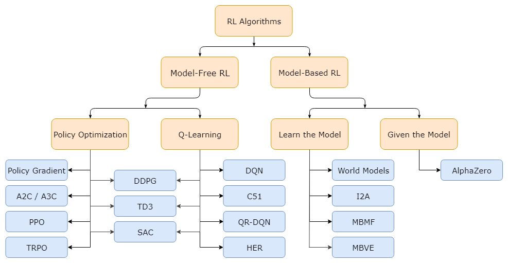
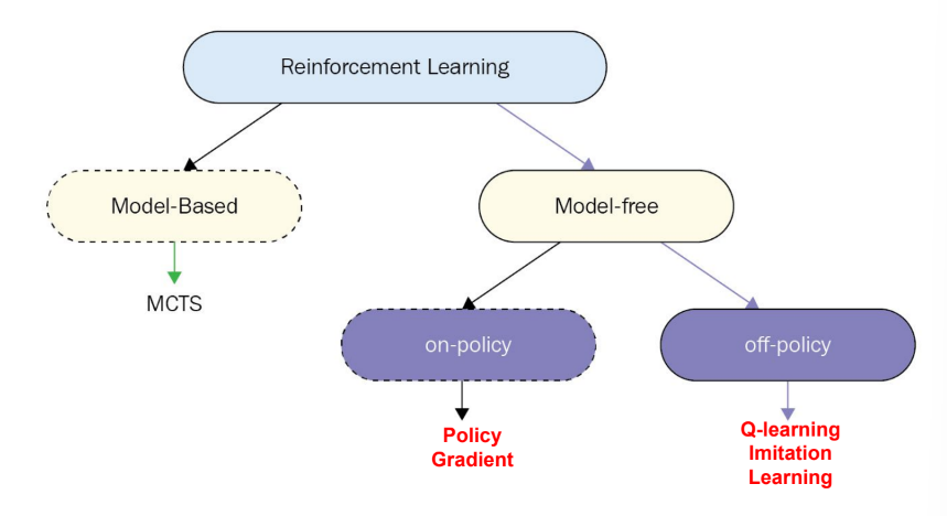
Taxonomy of RL algorithm

여기서

• Policy Optimization : on-policy RL
• Q-Learning : off-policy RL

Off-policy vs. On-policy

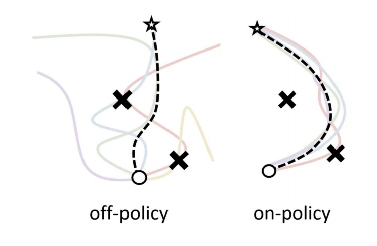
Policy Gradient is On-policy

algorithm

1. sample $\{\gamma^i\}$ from $\pi (a_t|s_t)$ (run it on the robot)
   skip 불가능!
2. $\bigtriangledown_\theta J(\theta) \approx \sum_i (\sum_t \bigtriangledown_\theta \log \pi_\theta (a_t^i|s_t^i)) (\sum_t r(s_t^i,a_t^i))$
3. $\theta \leftarrow \theta + \alpha\bigtriangledown_\theta J(\theta)$

pros

• 논리적으로는 언젠가 수렴한다는 것을 보장

cons

• Neural networks는 각 gradient step마다 조금씩만 변화
  $\because$ NN은 non-linear해서 크게 변화하면 optimize가 불가능해짐
• On-policy learning은 extremely inefficient해질 수 있음
  위의 이유로 인해서

Off-policy learning & importance sampling

sampling from the different distribution을 하고자 함

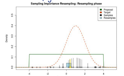
이렇게 density가 높은 부분을 더 많이 샘플링 하려고 함

importance sampling

$E_{x\sim p(x)}[f(x)] = \int p(x)f(x)dx \\ \quad\quad\quad\quad\space\space\space\quad= \int\frac{q(x)}{q(x)}p(x)f(x)dx \\ \quad\quad\quad\quad\quad\space\space\space = \int q(x)\frac{p(x)}{q(x)}f(x)dx \\ \quad\quad\quad\space\space\space\quad\quad= E_{x\sim q(x)} \big[\frac{p(x)}{q(x)} f(x)\big]$

이 importance sampling을 통해
different distribution을 sample함

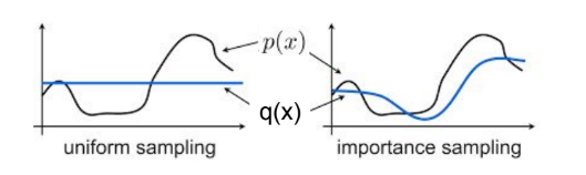
이렇게 uniform sampling과 달리 importance sampling은 $p(x)$의 모양을 따라서 sampling함
$p(x)$가 높은 부분이 더 sampling되도록
이때, $p(x)$는 original distribution that we want to learn

Policy gradient에 적용

objective function of policy gradient

$\theta^* = \underset{\theta}{\mathrm{argmax}}J(\theta)$
$J(\theta) = E_{\tau\sim p_\theta(\tau)}[r(\tau)]$

우리가 만약 $p_\theta(\tau)$에 대한 샘플을 가지고 있지 않으면 어떡할까?
And we have samples from some $\bar{p}(\tau)$ instead
$\bar{p}(\tau): q(x)$ - importance sampling distribution

importance sampling 식 사용해서 objective function 변경

$J(\theta) = E_{\tau\sim\bar{p}(\tau)}\big[\frac{p_\theta(\tau)}{\bar{p}(\tau)}r(\tau)\big]$

$p_\theta(\tau) = p(s_1)\underset{t=1}{\overset{T}\Pi}\pi_\theta(a_t|s_t)p(s_{t+1}|s_t,a_t)$

$\frac{p_\theta(\tau)}{\bar{p}(\tau)} = \frac{p(s_1)\underset{t=1}{\overset{T}\Pi}\pi_\theta(a_t|s_t)p(s_{t+1}|s_t,a_t)}{ p(s_1)\underset{t=1}{\overset{T}\Pi}\bar{\pi}(a_t|s_t)p(s_{t+1}|s_t,a_t)} = \frac{\underset{t=1}{\overset{T}\Pi}\pi_\theta(a_t|s_t)}{\underset{t=1}{\overset{T}\Pi}\bar{\pi}(a_t|s_t)}$
$\bar{\pi}$ : policy that we are sampling on
약분된 부분들은 같은 environmnet에서 왔으니 같은 값들이라서 cancle될 수 있었던 것임 수 있었던 것임

다시 최종 식을 보자면,

• 분모 : importance sampling에 따른 poicy
• 분자 : 우리가 끌어내고 싶은 policy

Deriving policy gradient with importance sampling

$J(\theta) = E_{\tau\sim\bar{p}(\tau)}\big[\frac{p_\theta(\tau)}{\bar{p}(\tau)}r(\tau)\big]$

위의 식에서 새로운 파라미터 $\theta'$를 estimate하는 방법

$J(\theta') = E_{\tau\sim p_\theta(\tau)}\big[\frac{p_{\theta'}(\tau)}{p_\theta(\tau)}r(\tau)\big]$
$p_{\theta'}(\tau)$ : the only bit that depends on $\theta'$ that is the off-policy policy gradient parameter

$\bigtriangledown_{\theta'}J(\theta') = E_{\tau\sim p_\theta(\tau)}\big[\frac{\bigtriangledown_{\theta'}p_{\theta'}(\tau)}{p_\theta(\tau)}r(\tau)\big] = E_{\tau\sim p_\theta(\tau)}\big[\frac{p_{\theta'}(\tau)\bigtriangledown_{\theta'}\log p_\theta(\tau)}{p_\theta(\tau)}r(\tau)\big]$
$\theta = \theta'$이 되는 경우 약분 가능

The off-policy policy gradient

$\bigtriangledown_{\theta'}J(\theta') = E_{\tau\sim p_\theta(\tau)}\big[\frac{p_{\theta'}(\tau)\bigtriangledown_{\theta'}\log p_\theta(\tau)}{p_\theta(\tau)}r(\tau)\big] \quad \text{when} \space \theta\neq\theta' \\ \quad\quad\quad\quad = E_{\tau\sim p_\theta(\tau)}\big[(\underset{t=1}{\overset{T}{\Pi}}\frac{\pi_{\theta'}(a_t|s_t)}{\pi_\theta(a_t|s_t)})(\underset{t=1}{\overset{T}{\sum}}\bigtriangledown_{\theta'}\log \pi_{\theta'}(a_t|s_t))(\underset{t=1}{\overset{T}{\sum}}r(s_t,a_t))\big]$

causality 적용하면
$\bigtriangledown_{\theta'}J(\theta') = E_{\tau\sim p_\theta(\tau)}\big[\underset{t-1}{\overset{T}{\sum}}\bigtriangledown_{\theta'}\log\pi_{\theta'}(a_t|s_t)(\underset{t'=1}{\overset{t}{\Pi}}\frac{\pi_{\theta'}(a_{t'}|s_{t'})}{\pi_\theta(a_{t'}|s_{t'})})(\underset{t'=t}{\overset{T}{\sum}}r(s_{t'}, a_{t'})(\underset{t''=t}{\overset{t'}{\Pi}}\frac{\pi_{\theta'}(a_{t''}|s_{t''})}{\pi_\theta(a_{t''}|s_{t''})}))\big]$

• $\underset{t'=1}{\overset{t}{\Pi}}\frac{\pi_{\theta'}(a_{t'}|s_{t'})}{\pi_\theta(a_{t'}|s_{t'})}$ : future actions don't affect current weight 반영
• $\underset{t''=t}{\overset{t'}{\Pi}}\frac{\pi_{\theta'}(a_{t''}|s_{t''})}{\pi_\theta(a_{t''}|s_{t''})}$ : 이 항을 무시하면, policy iteration algorithm을 얻게 됨

그런데 밑의 식에서,
$\bigtriangledown_{\theta'}J(\theta') = E_{\tau\sim p_\theta(\tau)}\big[\underset{t=1}{\overset{T}{\sum}}\bigtriangledown_{\theta'}\log \pi_{\theta'}(a_t|s_t)(\underset{t=1}{\overset{T}{\Pi}}\frac{\pi_{\theta'}(a_t|s_t)}{\pi_\theta(a_t|s_t)})(\underset{t=1}{\overset{T}{\sum}}r(s_t,a_t))\big]$

$\frac{\pi_{\theta'}(a_t|s_t)}{\pi_\theta(a_t|s_t)} < 1$이기 때문에, 계속 곱하다보면 값이 엄청 작아지게 됨
$\theta$에서 sampling하기 때문에 $\pi_\theta$가 $\pi_{\theta'}$보다 클 수밖에 없음
→ trajectory가 길다면, 뒤의 action은 gradient가 잘 흘러가지 못하게 됨

let's write the objective a bit differently

• on-policy policy gradient
  $\space \bigtriangledown_\theta J(\theta) \approx \frac{1}{N}\underset{i=1}{\overset{N}{\sum}}\underset{t=1}{\overset{T}{\sum}}\bigtriangledown_\theta\log\pi_\theta(a_{i,t}|s_{i,t})\hat{Q}_{i,t}$
• off-policy policy gradient
  $\space \bigtriangledown_{\theta'} J(\theta') \approx \frac{1}{N}\underset{i=1}{\overset{N}{\sum}}\underset{t=1}{\overset{T}{\sum}} \frac{\pi_{\theta'}(s_{i,t}, a_{i,t})}{\pi_\theta(s_{i,t}, a_{i,t})} \bigtriangledown_{\theta'}\log\pi_{\theta'}(a_{i,t}|s_{i,t})\hat{Q}_{i,t} \\ \quad\quad\quad\quad\ \approx \frac{1}{N}\underset{i=1}{\overset{N}{\sum}}\underset{t=1}{\overset{T}{\sum}}\frac{\pi_{\theta'}(s_{i,t})}{\pi_\theta(s_{i,t})}\frac{\pi_{\theta'}(a_{i,t}|s_{i,t})}{\pi_{\theta}(a_{i,t}|s_{i,t})}\bigtriangledown_{\theta'}\log\pi_{\theta'}(a_{i,t}|s_{i,t})\hat{Q}_{i,t}$
  • 이때, suppose $\pi_{\theta'}(s_t) = \pi_\theta(s_t)$ and ignore $\frac{\pi_{\theta'}(s_{i,t})}{\pi_\theta(s_{i,t})}$
    sometimes work in practice, when important sampling has same state distribution with the policy