6. Actor-Critic Design Decisions

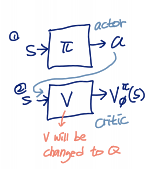
Actor-critic Design Decisions

Architecture Design

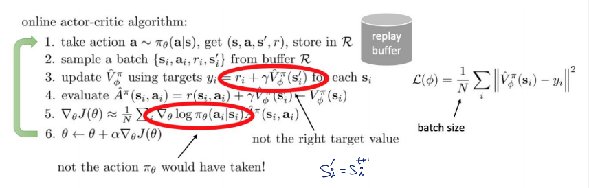
online actor-crotoc algorithm

1. take action $a\sim \pi_\theta(a|s)$, get $(s,a,s',r)$
2. update $\hat{V}_\phi^\pi$ using target $r+\gamma\hat{V}_\phi^\pi(s')$
3. evaluate $\hat{A}^\pi(s_i,a_i) = r(s_i,a_i)+\gamma\hat{V}_\phi^\pi(s_i')-\hat{V}_\phi^\pi(s_i)$
   $s_i' = s_{i+1}$
4. $\bigtriangledown_\theta J(\theta)\approx\underset{i}{\sum}\bigtriangledown_\theta\log\pi_\theta(a_i|s_i)\hat{A}^\pi(s_i,a_i)$
5. $\theta\leftarrow\theta+\alpha\bigtriangledown_\theta J(\theta)$

여기서 학습해야 하는 것은 두 개

1. policy function : actor
2. value function : critic
   

이 두 개를 학습하기 위한 디자인은 두 개가 있는데..

1. two network design

two different networks에서 $\hat{V}_\phi^\pi(s)$와 $\pi_\theta(a|s)$ 각각 학습

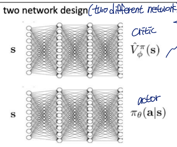
• 장점
  simple & stable
• 단점
  no shared features between actor & critic
  두 network 모두 s를 input으로 받는다는 공통점이 있지만 shared feature 없음

2. shared network design

하나의 network로 두 개 모두 학습

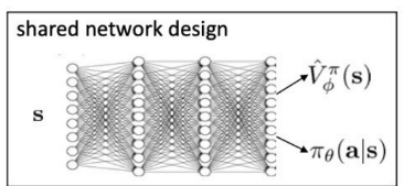
• 장점
  parameter memory 절감
  학습이 더 빨라지기도 함
• 단점
  unstable training

Online Actor-critic in practice

online actor-critic algorithm의 과정에서

2. update $\hat{V}_\phi^\pi$ using target $r+\gamma\hat{V}_\phi^\pi(s')$

를 수행할 때에는 works best with a batch (e.g., parallel workers)
예를 들어서 batch size가 16이면 16 workers를 사용 $\rightarrow$ 16 transition per 1 time 생성 가능

이때, worker를 사용하는 방법은 두 가지가 있음

1. synchronized parallel actor-critic
   
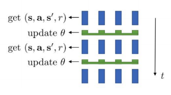
   모든 worker가 일을 끝낼 때까지 이미 일을 끝낸 worker도 다음 step으로 넘어가지 못함
   parameter를 optimize할 때에는 loss의 평균 사용

2. asynchronous parallel actor-critic
   
   각 에이전트가 독립적으로 학습하고 비동기적으로 업데이트(worker들은 parameter 공유)
   synchronized 때보다 학습 더 빨라짐
   그러나 일관적이지 못할 수도 있다는 단점 보유

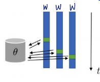
Can we remove the on-policy assumption entirely?

form a batch by using old previously seen transitions
이전에 경험한 state, action, reward, next state의 튜플(transition)을 사용하여 배치 형성

Off-Policy Learning은 현재의 정책이 아닌 이전의 정책에서 수집된 경험을 사용할 수 있기 때문에, 다양한 정책에 대한 학습이 가능해짐

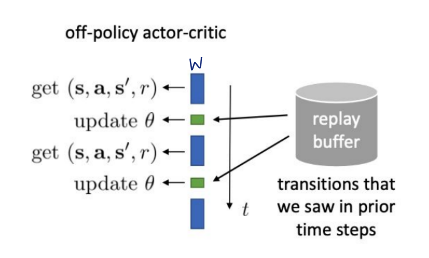
replay buffer에 과거의 transitions를 저장하고 후에 꺼내서 사용

그러나 이걸 진행하면 알고리즘에 붕괴가 발생함
이전의 transition은 old policy를 따르는 것인데, V에서는 현재의 policy를 따르는 transition을 사용해야 함. 따라서 gradient에 붕괴 발생
A should be sampled by current policy. 그러나 replay buffer에서 꺼낸 transition은 옛날 policy에서 sampled 된 것

이런 느낌

Fixing the policy update

V에는 A가 current policy를 따라야 한다는 assuption이 있기 때문에 이러한 가정이 없는 Q로 대체
$Q^\pi(s_t,a_t) = \underset{t'=t}{\overset{T}{\sum}}E_{\pi_\theta}[r(s_{t'},a_{t'})|s_t,a_t]$
여기서 $a_t$는 current policy를 따라야 함

따라서 알고리즘에서 3번은 이렇게 변함

3. update $\hat{Q}_\phi^\pi$ using targets $y_i = r_i+\gamma\hat{V}_\phi^\pi(s_i')$ for each $s_i,a_i\\\quad\quad\quad\quad\quad\quad\quad\quad\quad\quad\space\space=r_i+\gamma\hat{Q}_\phi^\pi(s_i',a_i')$
   
   $(s_i',a_i')$은 not from replay buffer R!$\quad a_i'\sim\pi_\theta(a_i'|s_i')$

이렇게 a는 current policy에서 예측하도록 만듦
$\rightarrow$ replay buffer에는 s, r만 있어도 되게 됨

그리고 policy의 loss function에도 변화 생김

$\bigtriangledown_\theta J(\theta) \approx \frac{1}{N}\underset{i}{\sum}\bigtriangledown_\theta\log\pi_\theta(a_i^\pi|s_i)Q^\pi(s_i,a_i^\pi)$
policy에서의 a도 replay buffer R에도 온 것 아님

$\hat{Q}^\pi(s_i,a_i^\pi)$: higher variance, but convenient
why is higher variance OK here? - sample 효율성, exploration,...

Some implementation details

위에서 바뀐 부분들을 알고리즘에 적용하면 최종적으로 이렇게 됨

1. take action $a\sim \pi_\theta(a|s)$, get $(s,a,s',r)$
2. sample a batch ${s_i,a_i,r_i,s_i'}$ from buffer R
3. update $\hat{Q}_\phi^\pi$ using targets $y_i = r_i+\gamma\hat{Q}_\phi^\pi(s_i',a_i')$ for each $s_i,a_i$
   lots of fancier ways to fit Q-functions
4. $\bigtriangledown_\theta J(\theta)\approx\underset{i}{\sum}\bigtriangledown_\theta\log\pi_\theta(a_i^\pi|s_i)\hat{Q}^\pi(s_i,a_i^\pi)\quad\text{where}\quad a_i^\pi\sim\pi_\theta(a|s_i)$
   could also use reparameterization trick to better estimate the integral
5. $\theta\leftarrow\theta+\alpha\bigtriangledown_\theta J(\theta)$

Q function의 input은 policy network의 output인 action과 replay buffer에서 나온 state