
0. 데이터 소개와 분석 목적
-
DACON 신용카드 사용자 연체 예측 AI 경진대회

1.주제
- 신용카드 사용자 데이터를 보고 사용자의 대금 연체 정도를 예측하는 알고리즘 개발
2.배경
- 신용카드사는 신용카드 신청자가 제출한 개인정보와 데이터를 활용해 신용 점수를 산정합니다. 신용카드사는 이 신용 점수를 활용해 신청자의 향후 채무 불이행과 신용카드 대급 연체 가능성을 예측합니다.
- 현재 많은 금융업계는 인공지능(AI)를 활용한 금융 서비스를 구현하고자 합니다. 사용자의 대금 연체 정도를 예측할 수 있는 인공지능 알고리즘을 개발해 금융업계에 제안할 수 있는 인사이트를 발굴해주세요!
3.대회 설명
- 신용카드 사용자들의 개인 신상정보 데이터로 사용자의 신용카드 대금 연체 정도를 예측
데이터 변수
X Variables
-
index
-
gender: 성별(남,여)
-
car: 차량 소유 여부
-
reality: 부동산 소유 여부
-
child_num: 자녀 수
-
income_total: 연간 소득
-
income_type: 소득 분류
['Commercial associate', 'Working', 'State servant', 'Pensioner', 'Student'] -
edu_type: 교육 수준
['Higher education' ,'Secondary / secondary special', 'Incomplete higher', 'Lower secondary', 'Academic degree']- family_type: 결혼 여부
['Married', 'Civil marriage', 'Separated', 'Single / not married', 'Widow']- house_type: 생활 방식
['Municipal apartment', 'House / apartment', 'With parents', 'Co-op apartment', 'Rented apartment', 'Office apartment']- DAYS_BIRTH: 출생일 (데이터 수집 당시 (0)부터 역으로 셈, 즉, -1은 데이터 수집일 하루 전에 태어났음을 의미)
-
DAYS_EMPLOYED: 업무 시작일 (데이터 수집 당시 (0)부터 역으로 셈, 즉, -1은 데이터 수집일 하루 전부터 일을 시작함을 의미, 양수 값은 고용되지 않은 상태를 의미함)
-
FLAG_MOBIL: 핸드폰 소유 여부
-
work_phone: 업무용 전화 소유 여부
-
phone: 전화 소유 여부
-
email: 이메일 소유 여부
-
occyp_type: 직업 유형
-
family_size: 가족 규모
-
begin_month: 신용카드 발급 월 (데이터 수집 당시 (0)부터 역으로 셈, 즉, -1은 데이터 수집일 한 달 전에 신용카드를 발급함을 의미)
y Variable
- credit: 사용자의 신용카드 대금 연체를 기준으로 한 신용도 (0, 1, 2) (낮을 수록 높은 신용의 신용카드 사용자를 의미함)
1. R을 통한 데이터 탐색
# 데이터 불러오기
train = read.csv(".../Data/train.csv")
# 데이터 Structure 보기
str(train)
## 'data.frame': 26457 obs. of 20 variables:
## $ index : int 0 1 2 3 4 5 6 7 8 9 ...
## $ gender : chr "F" "F" "M" "F" ...
## $ car : chr "N" "N" "Y" "N" ...
## $ reality : chr "N" "Y" "Y" "Y" ...
## $ child_num : int 0 1 0 0 0 2 0 0 1 0 ...
## $ income_total : num 202500 247500 450000 202500 157500 ...
## $ income_type : chr "Commercial associate" "Commercial associate" "Working" "Commercial associate" ...
## $ edu_type : chr "Higher education" "Secondary / secondary special" "Higher education" "Secondary / secondary special" ...
## $ family_type : chr "Married" "Civil marriage" "Married" "Married" ...
## $ house_type : chr "Municipal apartment" "House / apartment" "House / apartment" "House / apartment" ...
## $ DAYS_BIRTH : int -13899 -11380 -19087 -15088 -15037 -13413 -17570 -14896 -15131 -15785 ...
## $ DAYS_EMPLOYED: int -4709 -1540 -4434 -2092 -2105 -4996 -1978 -5420 -1466 -1308 ...
## $ FLAG_MOBIL : int 1 1 1 1 1 1 1 1 1 1 ...
## $ work_phone : int 0 0 0 0 0 0 0 0 0 0 ...
## $ phone : int 0 0 1 1 0 0 0 0 0 0 ...
## $ email : int 0 1 0 0 0 1 1 1 1 0 ...
## $ occyp_type : chr "" "Laborers" "Managers" "Sales staff" ...
## $ family_size : num 2 3 2 2 2 4 1 2 3 2 ...
## $ begin_month : num -6 -5 -22 -37 -26 -18 -41 -53 -38 -5 ...
## $ credit : num 1 1 2 0 2 1 2 0 2 2 ...# factor 변수로 치환
train$gender = as.factor(train$gender)
train$car = as.factor(train$car)
train$reality = as.factor(train$reality)
train$income_type = as.factor(train$income_type)
train$edu_type = as.factor(train$edu_type)
train$family_type = as.factor(train$family_type)
train$house_type = as.factor(train$house_type)
train$FLAG_MOBIL = as.factor(train$FLAG_MOBIL)
train$work_phone = as.factor(train$work_phone)
train$phone = as.factor(train$phone)
train$email = as.factor(train$email)
train$occyp_type = as.factor(train$occyp_type)
## Y variable
train$credit = as.factor(train$credit)# 데이터 Summary 보기
summary(train)
## index gender car reality child_num
## Min. : 0 F:17697 N:16410 N: 8627 Min. : 0.0000
## 1st Qu.: 6614 M: 8760 Y:10047 Y:17830 1st Qu.: 0.0000
## Median :13228 Median : 0.0000
## Mean :13228 Mean : 0.4287
## 3rd Qu.:19842 3rd Qu.: 1.0000
## Max. :26456 Max. :19.0000
##
## income_total income_type
## Min. : 27000 Commercial associate: 6202
## 1st Qu.: 121500 Pensioner : 4449
## Median : 157500 State servant : 2154
## Mean : 187307 Student : 7
## 3rd Qu.: 225000 Working :13645
## Max. :1575000
##
## edu_type family_type
## Academic degree : 23 Civil marriage : 2123
## Higher education : 7162 Married :18196
## Incomplete higher : 1020 Separated : 1539
## Lower secondary : 257 Single / not married: 3496
## Secondary / secondary special:17995 Widow : 1103
##
##
## house_type DAYS_BIRTH DAYS_EMPLOYED FLAG_MOBIL
## Co-op apartment : 110 Min. :-25152 Min. :-15713 1:26457
## House / apartment :23653 1st Qu.:-19431 1st Qu.: -3153
## Municipal apartment: 818 Median :-15547 Median : -1539
## Office apartment : 190 Mean :-15958 Mean : 59069
## Rented apartment : 429 3rd Qu.:-12446 3rd Qu.: -407
## With parents : 1257 Max. : -7705 Max. :365243
##
## work_phone phone email occyp_type family_size
## 0:20511 0:18672 0:24042 :8171 Min. : 1.000
## 1: 5946 1: 7785 1: 2415 Laborers :4512 1st Qu.: 2.000
## Core staff :2646 Median : 2.000
## Sales staff:2539 Mean : 2.197
## Managers :2167 3rd Qu.: 3.000
## Drivers :1575 Max. :20.000
## (Other) :4847
## begin_month credit
## Min. :-60.00 0: 3222
## 1st Qu.:-39.00 1: 6267
## Median :-24.00 2:16968
## Mean :-26.12
## 3rd Qu.:-12.00
## Max. : 0.00-
현재 X variables 중에서 불필요해 보이는 variables 들은
index
FLAG_MOBILE : The variable has only one level.
phone
email
work_phone
-
값을 변환 할 변수
income_total
- 수입의 경우 Numerical 보단 소득분위에 따른 level 값으로 보는게 효율적이다. (예: 소득 10분위)
- 현재 income_total의 경우 단위가 정확하지 않기 때문에 주어진 데이터에서 소득 분위를 만드는 것이 효율적일 것으로 보인다.
DAYS_BIRTH
- 연령은 구간에 따른 EDA를 진행하는것이 효율적일 것으로 보인다.
begin_month
- 신용카드 사용한 연수로 보는게 효율적일 것으로 보인다.
DAYS_EMPLOYED
- 근무 연수로 보는게 효율적일 것으로 보인다.
-
고려해봐야 할 변수
edu_type: 변수의 Secondary/secondary special에 17,995명이 기입되어 있다.
- 대한민국의 평균적인 교육 수준을 고려했을시 변수에 중졸 비율이 높아 보인다.
- 고객이 학력을 입력하지 않았을시 Default로 중등교육으로 입력될 가능성이 있다.
occyp_type: 19개의 level이 있고 NA 값이 8,171개 존재한다.
- $ occyp_type: Factor w/ 19 levels "","Accountants",..: 1 10 12 16 12 7 5 6 1 13 ...
2. EDA Setting
2.1 Library 불러오기
import pandas as pd
import numpy as np
import matplotlib.pyplot as plt
import seaborn as sns
# seaborn setting
sns.set_theme(style='whitegrid')
sns.set_palette("twilight")import scipy.stats as stats2.2 데이터 불러오기
# 데이터 train에 지정하기
train = pd.read_csv('train.csv')
train.head(5)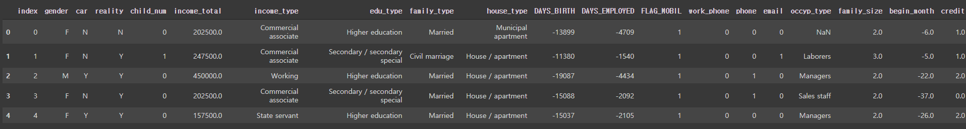
# 불필요한 변수 Drop
train.drop(columns=['index','FLAG_MOBIL','phone','email','work_phone', 'edu_type'], inplace=True)
train.head(3)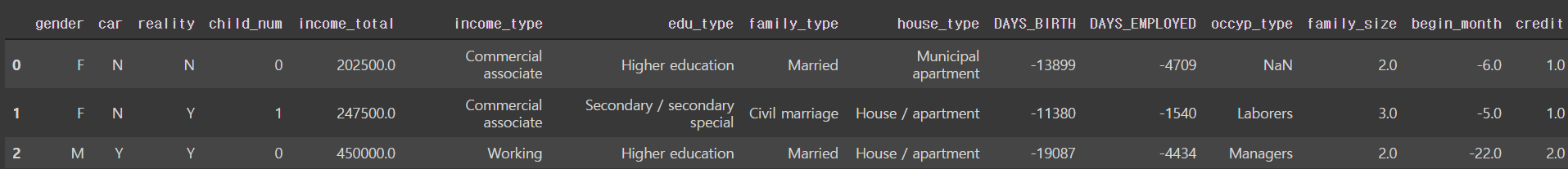
train.info()
## occyp_type에 NULL 값이 존재한다.
<class 'pandas.core.frame.DataFrame'>
RangeIndex: 26457 entries, 0 to 26456
Data columns (total 15 columns):
 #   Column         Non-Null Count  Dtype
---  ------         --------------  -----
 0   gender         26457 non-null  object
 1   car            26457 non-null  object
 2   reality        26457 non-null  object
 3   child_num      26457 non-null  int64
 4   income_total   26457 non-null  float64
 5   income_type    26457 non-null  object
 6   edu_type       26457 non-null  object
 7   family_type    26457 non-null  object
 8   house_type     26457 non-null  object
 9   DAYS_BIRTH     26457 non-null  int64
 10  DAYS_EMPLOYED  26457 non-null  int64
 11  occyp_type     18286 non-null  object
 12  family_size    26457 non-null  float64
 13  begin_month    26457 non-null  float64
 14  credit         26457 non-null  float64
dtypes: float64(4), int64(3), object(8)
memory usage: 3.0+ MB
train.describe(include='all')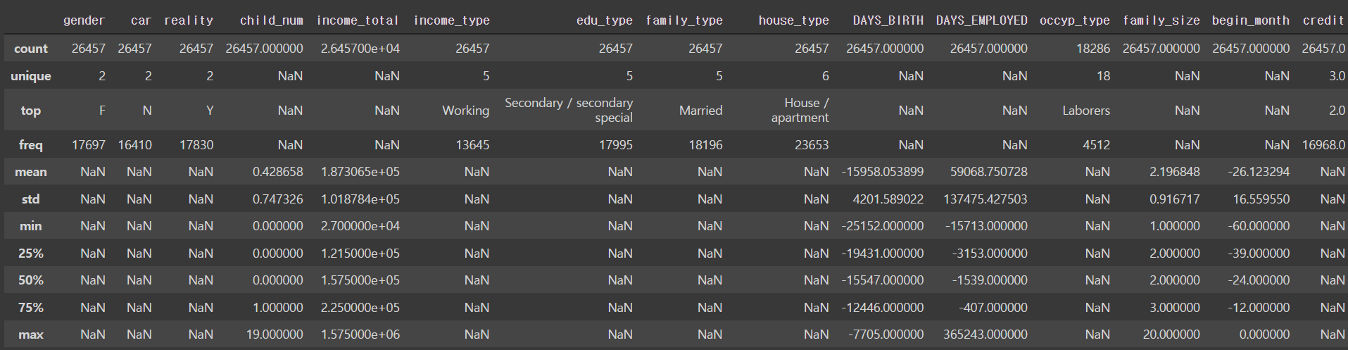
2.3 연간 소득 분위 값 할당
# income_total 에 대한 QQ-plot그리기
plt.figure(figsize=(10, 8))
stats.probplot(train['income_total'], dist=stats.norm, plot=plt)
plt.show()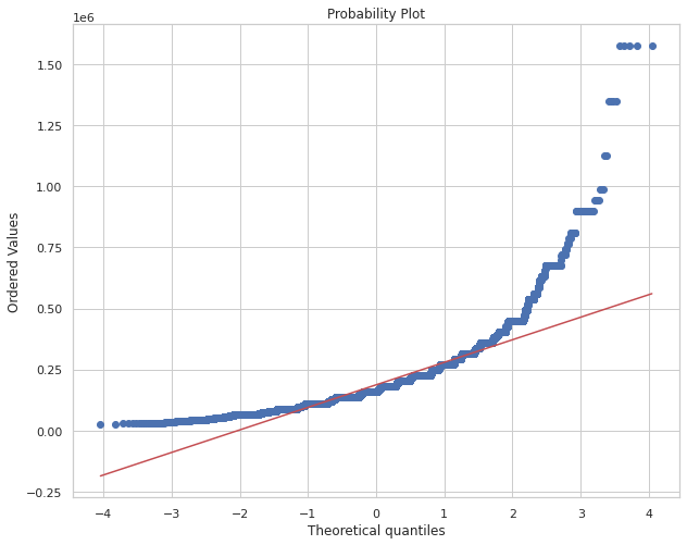
- 현재 income_total에 대한 QQ-plot을 보면 대부분 데이터의 수입 QQ-plot과 마찬가지로 linear 형식보단 right-skewed 형식을 보영준다.
- 소득분위에 대해 4, 5, 10분위로 나눈 후 후에 모델링에서 어떠한 값이 더 효율적인 확인후 사용하자.
# variable 'income_quintile' 생성
train['income_quartile'] = np.zeros(26457)
# variable 'income_quintile' 생성
train['income_quintile'] = np.zeros(26457)
# variable 'income_decile' 생성
train['income_decile'] = np.zeros(26457)
# income_quartile에 값 할당하기
train['income_quartile'][train['income_total'] < train['income_total'].quantile(0.25)] = 1
train['income_quartile'][(train['income_total'] >= train['income_total'].quantile(0.25)) &
(train['income_total'] < train['income_total'].quantile(0.5))] = 2
train['income_quartile'][(train['income_total'] >= train['income_total'].quantile(0.5)) &
(train['income_total'] < train['income_total'].quantile(0.75))] = 3
train['income_quartile'][train['income_total'] >= train['income_total'].quantile(0.75)] = 4# income_quintile에 값 할당하기
train['income_quintile'][train['income_total'] < train['income_total'].quantile(0.2)] = 1
train['income_quintile'][(train['income_total'] >= train['income_total'].quantile(0.2)) &
(train['income_total'] < train['income_total'].quantile(0.4))] = 2
train['income_quintile'][(train['income_total'] >= train['income_total'].quantile(0.4)) &
(train['income_total'] < train['income_total'].quantile(0.6))] = 3
train['income_quintile'][(train['income_total'] >= train['income_total'].quantile(0.6)) &
(train['income_total'] < train['income_total'].quantile(0.8))] = 4
train['income_quintile'][train['income_total'] >= train['income_total'].quantile(0.8)] = 5# income_decile에 값 할당하기
train['income_decile'][train['income_total'] < train['income_total'].quantile(0.1)] = 1
train['income_decile'][(train['income_total'] >= train['income_total'].quantile(0.1)) &
(train['income_total'] < train['income_total'].quantile(0.2))] = 2
train['income_decile'][(train['income_total'] >= train['income_total'].quantile(0.2)) &
(train['income_total'] < train['income_total'].quantile(0.3))] = 3
train['income_decile'][(train['income_total'] >= train['income_total'].quantile(0.3)) &
(train['income_total'] < train['income_total'].quantile(0.4))] = 4
train['income_decile'][(train['income_total'] >= train['income_total'].quantile(0.4)) &
(train['income_total'] < train['income_total'].quantile(0.5))] = 5
train['income_decile'][(train['income_total'] >= train['income_total'].quantile(0.5)) &
(train['income_total'] < train['income_total'].quantile(0.6))] = 6
train['income_decile'][(train['income_total'] >= train['income_total'].quantile(0.6)) &
(train['income_total'] < train['income_total'].quantile(0.7))] = 7
train['income_decile'][(train['income_total'] >= train['income_total'].quantile(0.7)) &
(train['income_total'] < train['income_total'].quantile(0.8))] = 8
train['income_decile'][(train['income_total'] >= train['income_total'].quantile(0.8)) &
(train['income_total'] < train['income_total'].quantile(0.9))] = 9
train['income_decile'][train['income_total'] >= train['income_total'].quantile(0.9)] = 10train.info()
<class 'pandas.core.frame.DataFrame'>
RangeIndex: 26457 entries, 0 to 26456
Data columns (total 18 columns):
# Column Non-Null Count Dtype
--- ------ -------------- -----
0 gender 26457 non-null object
1 car 26457 non-null object
2 reality 26457 non-null object
3 child_num 26457 non-null int64
4 income_total 26457 non-null float64
5 income_type 26457 non-null object
6 edu_type 26457 non-null object
7 family_type 26457 non-null object
8 house_type 26457 non-null object
9 DAYS_BIRTH 26457 non-null int64
10 DAYS_EMPLOYED 26457 non-null int64
11 occyp_type 18286 non-null object
12 family_size 26457 non-null float64
13 begin_month 26457 non-null float64
14 credit 26457 non-null float64
15 income_quartile 26457 non-null float64
16 income_quintile 26457 non-null float64
17 income_decile 26457 non-null float64
dtypes: float64(7), int64(3), object(8)
memory usage: 3.6+ MB2.4 연령별 그룹 생성
# age 변수 생성
# DAYS_BIRTH에 -1곱하고 365로 나누고 몫에다 +1
train['age'] = (train['DAYS_BIRTH'] * (-1))//365+1
# age_group 변수 생성
train['age_group'] = np.zeros(26457)
train['age'].describe()
count 26457.000000
mean 44.213478
std 11.513590
min 22.000000
25% 35.000000
50% 43.000000
75% 54.000000
max 69.000000
Name: age, dtype: float64# 29Under, 30~39, 40~49, 50~64, 65+ 구간으로 나누어 주자
train['age_group'][train['age']<30] = '20s'
train['age_group'][(train['age']>=30) & (train['age']<40)] = '30s'
train['age_group'][(train['age']>=40) & (train['age']<50)] = '40s'
train['age_group'][(train['age']>=50) & (train['age']<60)] = '50s'
train['age_group'][train['age']>=60] = '60s'2.5 신용카드 사용 연수
# 신용카드 사용 연수 생성
# -1 곱해주고 12 나누고 내림
train['used_years'] = train['begin_month']*(-1)//12

train['used_years'] = train['used_years'].astype('int')
2.6 근무 연수
# worked_year 변수지정
train['worked_year'] = train['DAYS_EMPLOYED']*(-1)

# 취업되지 않은 사람들에 대해 -365 지정
train['worked_year'][train['worked_year']<0] = -365

# 근무연수를 구하기 위해 worked_year를 365로 나누고 몫만 지정
# 근무연수가 없는 사람들은 -1에 지정
train['worked_year'] = train['worked_year']//365
train.head(3)