
3. 성별, 연령, 신용카드 이용 연수에 대한 EDA
3.1 성별에 따른 EDA
# 성별에 따른 신용등급 인원수
pd.crosstab(train['gender'], train['credit'], margins=True, margins_name='Total')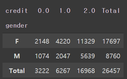
- 여성고객이 남성고객보다 많다.
# 성별에 따른 신용등급 비율
pd.crosstab(train['gender'], train['credit'], normalize='index')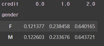
- 성별에 따른 신용등급은 큰 차이를 보이지 않는다.
3.2 연령에 따른 EDA
# 연령에 따른 신용등급 인원수
pd.crosstab(train['age_group'], train['credit'], margins=True, margins_name='Total')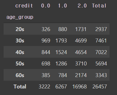
# 연령에 따른 신용등급 비율
pd.crosstab(train['age_group'], train['credit'], normalize='index')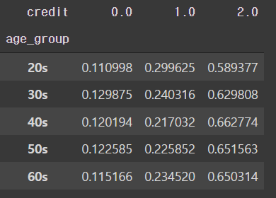
- 연령에 따른 신용 비율이 뚜렷이 보여주는 차이가 없다
3.3 신용카드 이용 연수에 따른 EDA
pd.crosstab(train['used_years'], train['credit'], margins=True, margins_name='Total')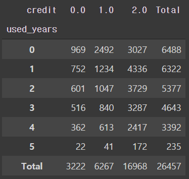
pd.crosstab(train['used_years'], train['credit'], normalize='index')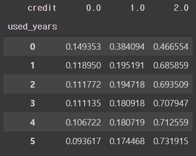
- 신용카드는 사용 연수가 증가 할 수록 신용등급률이 떨어지는 것으로 보인다.
- 신용카드 사용 첫번째 1년이 지날때 비율이 가장 많이 떨어지고 그 후엔 조금씩 지속적으로 떨어진다.
- 신용 2등급의 경우 처음 1년이 지나고 가장 많이 오른다.
3.4 성별과 연령, 사용 연수에 따른 종합적인 EDA
# 성별과 연령대에 따른 신용등급 인원수
pd.crosstab([train['gender'],train['age_group']], train['credit'])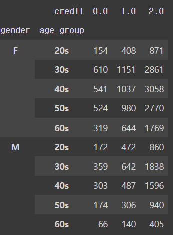
# 성별과 연령대에 따른 신용등급 비율
pd.crosstab([train['gender'],train['age_group']], train['credit'], normalize='index')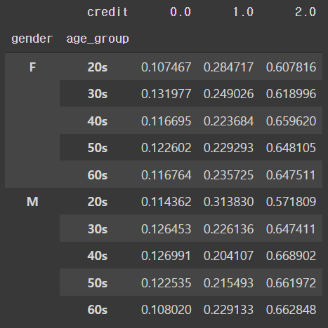
- 성별과 연령대에 따른 신용등급의 변화는 뚜렷이 보이는 것이 없다.
3.5 연령과 사용연수에 따른 EDA
# 연령대와 사용연수에 따른 신용등급 비율
pd.crosstab([train['age_group'],train['used_years']], train['credit'], normalize='index')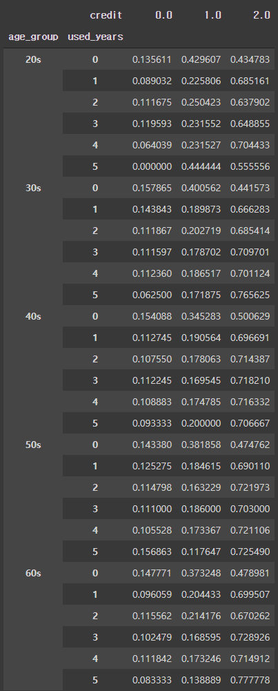
- 연령대에 따라 신용카드 이용연수가 증가 할 수록 신용등급 변화가 다르게 나타난다.
# heatmap에 따른 연령대와 사용연수에 따른 신용등급 비율
## 20s
twenty = train[train['age_group']=='20s']
twentyUsedYear = pd.crosstab([twenty['age_group'],twenty['used_years']], twenty['credit'], normalize='index')

## 30s
thirty = train[train['age_group']=='30s']
thirtyUsedYear = pd.crosstab([thirty['age_group'],thirty['used_years']], thirty['credit'], normalize='index')

## 40s
forty = train[train['age_group']=='40s']
fortyUsedYear = pd.crosstab([forty['age_group'],forty['used_years']], forty['credit'], normalize='index')

## 50s
fifty = train[train['age_group']=='50s']
fiftyUsedYear = pd.crosstab([fifty['age_group'],fifty['used_years']], fifty['credit'], normalize='index')

## 60s
sixty = train[train['age_group']=='60s']
sixtyUsedYear = pd.crosstab([sixty['age_group'],sixty['used_years']], sixty['credit'], normalize='index')
# 사이즈 지정
plt.figure(figsize=(20,10))
plt.subplot(2,3,1)
sns.heatmap(twentyUsedYear, vmin=0, vmax=0.8,
linewidths=1, cmap="seismic_r", cbar=False)
plt.subplot(2,3,2)
sns.heatmap(thirtyUsedYear, vmin=0, vmax=0.8,
linewidths=1, cmap="seismic_r", cbar=False)
plt.subplot(2,3,3)
sns.heatmap(fortyUsedYear, vmin=0, vmax=0.8,
linewidths=1, cmap="seismic_r", cbar=False)
plt.subplot(2,3,4)
sns.heatmap(fiftyUsedYear, vmin=0, vmax=0.8,
linewidths=1, cmap="seismic_r", cbar=False)
plt.subplot(2,3,5)
sns.heatmap(sixtyUsedYear, vmin=0, vmax=0.8,
linewidths=1, cmap="seismic_r", cbar=False)
plt.show()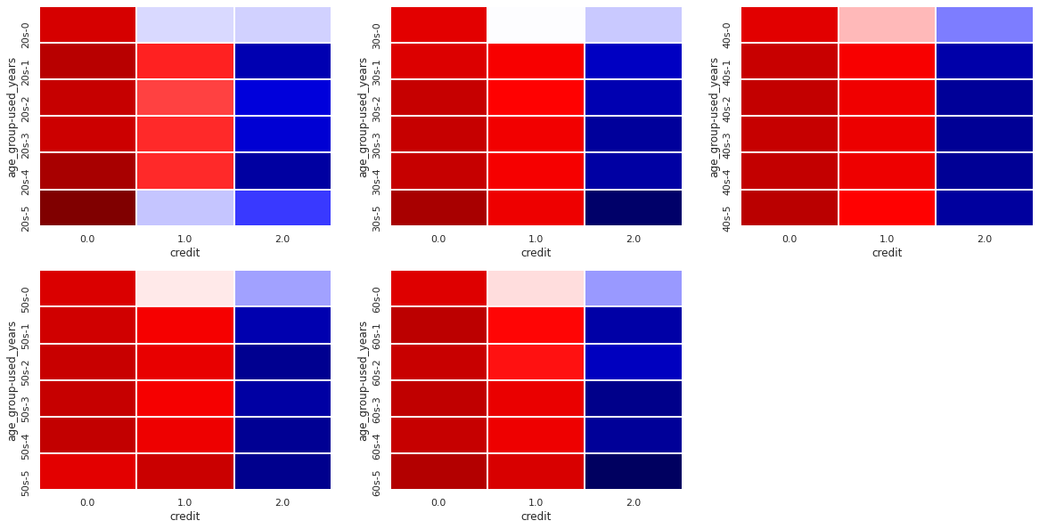
- 짙은 감색일 수록 비율이 높고 짙은 적색일 수록 비율이 낮다.
- 위에 테이블에서 보여준 숫자 상으론 차이가 보이긴 하나 명확하게 어떠한 차이가 있는지 보이지 않는다.
- 후에 modeling을 통한 수치 비교를 해야 할거 같다.
4. 실물 자산에 따른 EDA
4.1 부동산 소유에 따른 신용등급
# 부동산 소유에 따른신용등급 인원수
pd.crosstab(train['reality'], train['credit'], margins=True, margins_name='Total')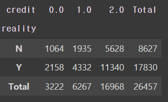
- 신용카드 사용자 중 대부분은 부동산을 소유하고 있다.
# 부동산 소유에 따른신용등급 비율
pd.crosstab(train['reality'], train['credit'], normalize='index')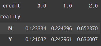
- 비율상 두 level의 차이는 크게 다르지 않다.
4.2 부동산 종류에 따른 신용등급
# 부동산 종류에 따른신용등급 인원수
pd.crosstab(train['house_type'], train['credit'], margins=True, margins_name='Total')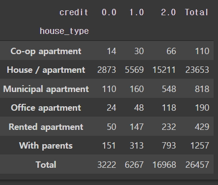
- 대부분의 경우 아파트에 거주하고 있다.
# 부동산 종류에 따른신용등급 비율
pd.crosstab(train['house_type'], train['credit'], normalize='index')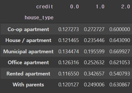
- 비율 상으로 크게 차이가 나는 level은 보이지 않는다.
- Municipal apaetment에 거주 하는 사람들의 경우 신용등급 0과 1의 비율차가 다른 level에 비해 많이 나진 않는다.
- 그러나 Municipal apaetment의 경우 신용등급 2의 비율이 가장 높다.
4.3 자동차 소유에 따른 신용등급
# 자동차 소유에 따른신용등급 인원수
pd.crosstab(train['car'], train['credit'], margins=True, margins_name='Total')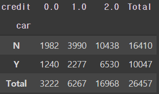
- 자동차를 소유하고 있지 않은 고객이 더 많다.
# 자동차 소유에 따른신용등급 비율
pd.crosstab(train['car'], train['credit'], normalize='index')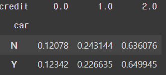
- 비율적으로 큰 차이가 보이진 않는다.
4.4 연령과 자동차 소유에 대한 신용등급
- 가정: 20대 승용차를 가지고 있을 경우 무리해서 구매 했을 가능성이 있다.
- 따라서 20대 경우 승용차를 소유 하고 있는 그룹과 아닌 그룹간의 차이를 보여줄 수 있다.
# 20대의 차량 소유에 따른 신용등급 비율
pd.crosstab(twenty['car'], twenty['credit'], normalize='index')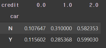
- 차량 소유에 따른 신용등급의 비율 차가 많이 나지 않는다
pd.crosstab([twenty['car'], twenty['used_years']], twenty['credit'], margins=True, margins_name='Total')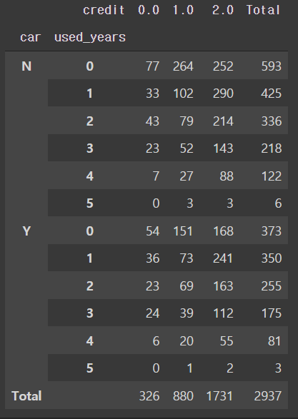
pd.crosstab([twenty['car'], twenty['used_years']], twenty['credit'], normalize='index')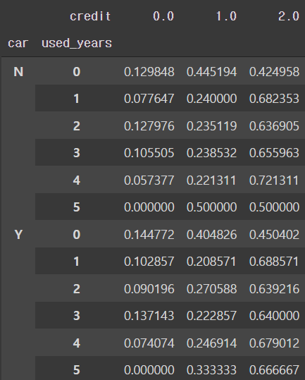
- 싱용카드 사용 연수에 따른 결과 값이 사이즈를 고려 했을시 의미있다 보긴 힘들다.
- 따라서 지금 단계에선 20대가 자동차를 소유했다고해서 신용등급이 영향을 받는다고 결론을 내리긴 힘들어 보인다.
5. 가족 정보에 따른 신용정보
5.1 가족 유형(family_type)에 따른 신용등급
# 가족 유형에 따른 신용등급 인원수
pd.crosstab(train['family_type'], train['credit'], margins=True, margins_name='Total')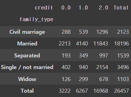
# 가족 유형에 따른 신용등급 비율
pd.crosstab(train['family_type'], train['credit'], normalize='index')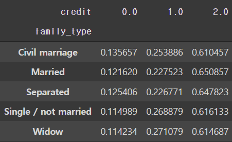
- civil marriage와 married의 경우 같은 값으로 봐도 괜찮을 수 있다.
5.1.1 가족 유형과 연령에 따른 비율과 인원수
pd.crosstab(train['family_type'], train['age_group'], margins=True, margins_name='Total')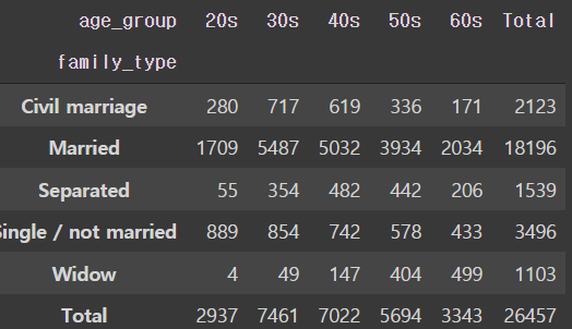
pd.crosstab(train['family_type'], train['age_group'], normalize='columns')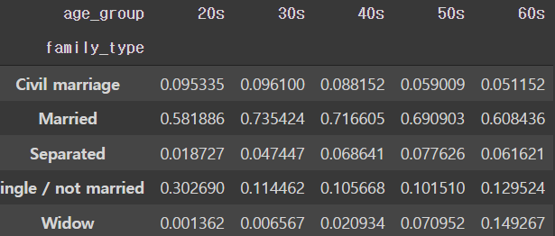
- 신용카드 회사의 주 고객층은 30대에서 50대 이다.
- 전 연령 층에서 결혼한 고객들의 비율이 가장 높다.
5.2 가족 인원수에 따른 신용등급
# 가족 인원수에 따른 신용등급
pd.crosstab(train['family_size'], train['credit'], margins='total', margins_name='Total')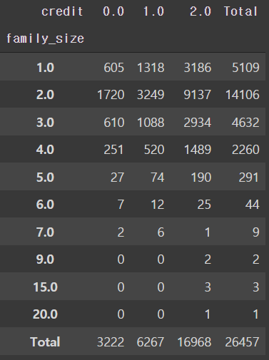
- 대부분의 고객은 2인가족이다.
- 5인 이상의 고객의 경우 데이터의 사이즈가 작다.
# 가족 인원 1~4명에 따른 신용등급 비율
pd.crosstab(train['family_size'][train['family_size'] < 5], train['credit'], normalize='index')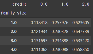
- 가족 인원수에 따른 신용등급의 유의미한 차이가 현재 보이지 않는다.
5.3 자녀에 따른 신용등급
# 자녀에 따른 신용등급
pd.crosstab(train['child_num'], train['credit'], margins='total', margins_name='Total')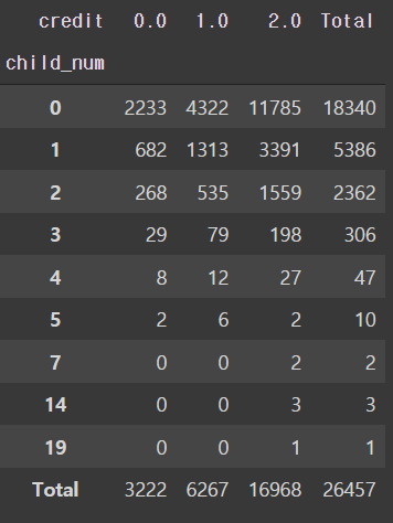
- 자녀가 3명 이하인 경우에 따른 비율을 보는것이 효율적일 것으로 보인다.
# 자녀에 따른 신용등급
pd.crosstab(train['child_num'][train['child_num']<4], train['credit'], normalize='index')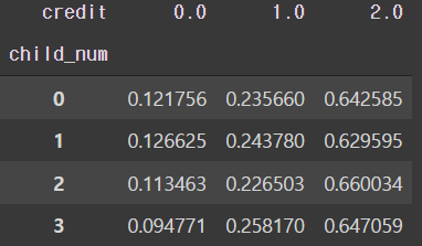
- 자녀가 3명인 경우 신용등급 0이 다른 그룹에 비해 낮다.
5.3.1 가족 유형과 자녀 명수에 따른 신용등급
# 자녀가 3명 이하인 경우에 따른 가족 유형 인원수
pd.crosstab(train['child_num'][train['child_num']<4], train['family_type'], margins='total', margins_name='Total')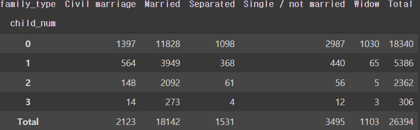
# 자녀가 3명 이하인 경우에 따른 가족 유형 인원수
pd.crosstab([train['family_type'], train['child_num'][train['child_num']<4]],
            train['credit'], margins='total', margins_name='Total')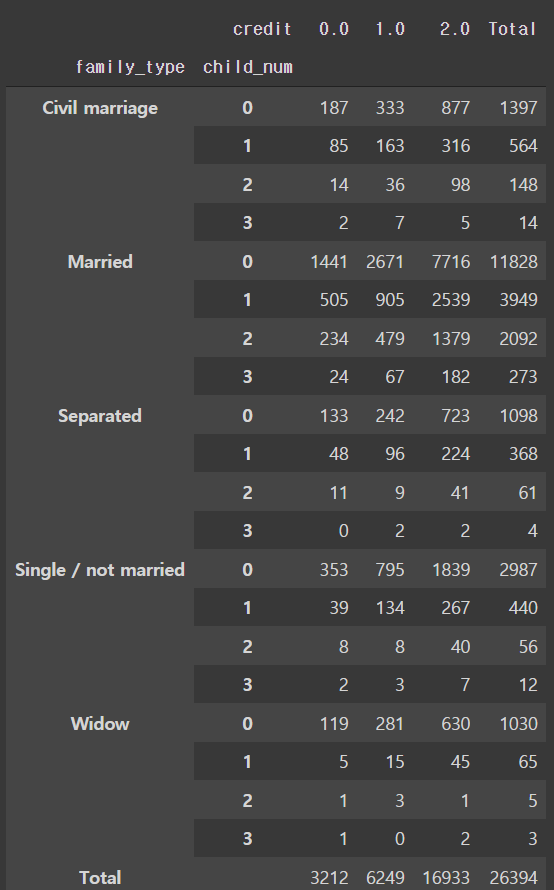
- 각 셀의 인원수를 고려 했을시 자녀수가 2명 이하인 경우가 유의미한 정보를 보여주는 것으로 보인다.
- 가족 유형은 결혼한 인원에 대해서만 보는게 효율적일 것으로 보인다.
6. 직장과 수입에 따른 신용등급
6.1 수입 방식에 따른 신용등급
# income_type에 따른 신용 등급 인원수
pd.crosstab(train['income_type'], train['credit'], margins='total', margins_name='Total')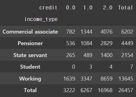
# income_type에 따른 신용 등급 비율
pd.crosstab(train['income_type'], train['credit'], normalize='index')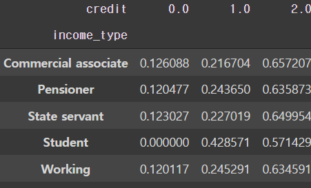
- 학생의 경우 절대적인 인원수가 적어 의미 있는 정보를 찾아보기 힘들다.(후에 학생에 대한 값들은 드롭하는 것이 좋을 수 있다.)
- 다른 변수들의 경우 비슷한 트렌드를 보인다.
6.2 수입에 따른 신용등급
# 4분위에 대한 정보
pd.crosstab(train['income_quartile'], train['credit'], normalize='index')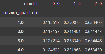
sns.displot(x='income_quintile', hue='credit', multiple='stack', col='credit', bins=4, data=train)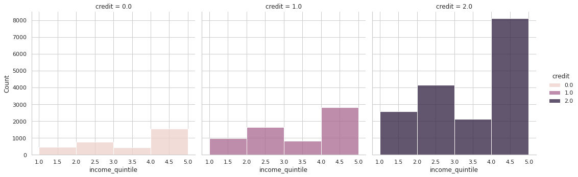
# 5분위에 대한 정보
pd.crosstab(train['income_quintile'], train['credit'], normalize='index')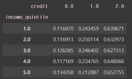
# 5분위에 따른 신용 등급
sns.displot(x='income_quintile', hue='credit', multiple='stack', col='credit', bins=5,data=train)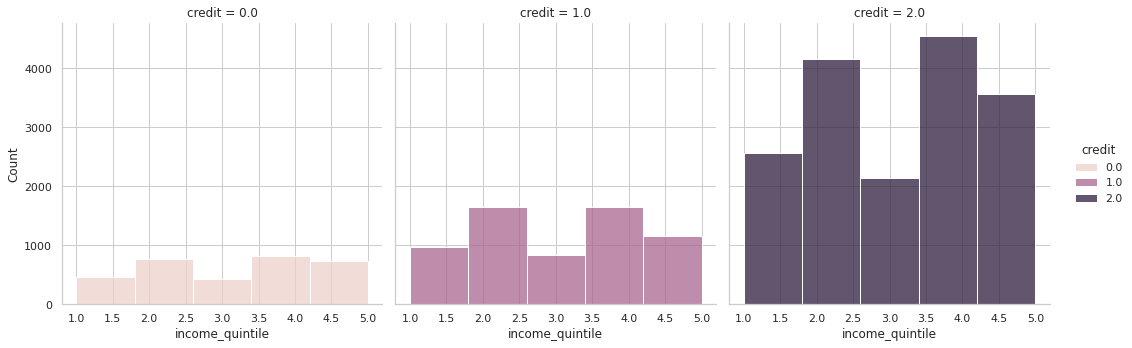
# 10분위에 대한 정보
pd.crosstab(train['income_decile'], train['credit'], normalize='index')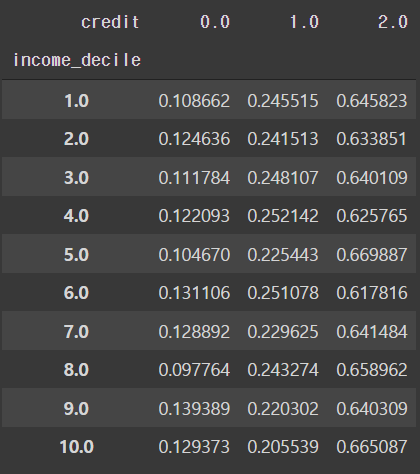
# 10분위에 따른 신용 등급
sns.displot(x='income_decile', hue='credit', multiple='stack', col='credit', bins=10,data=train)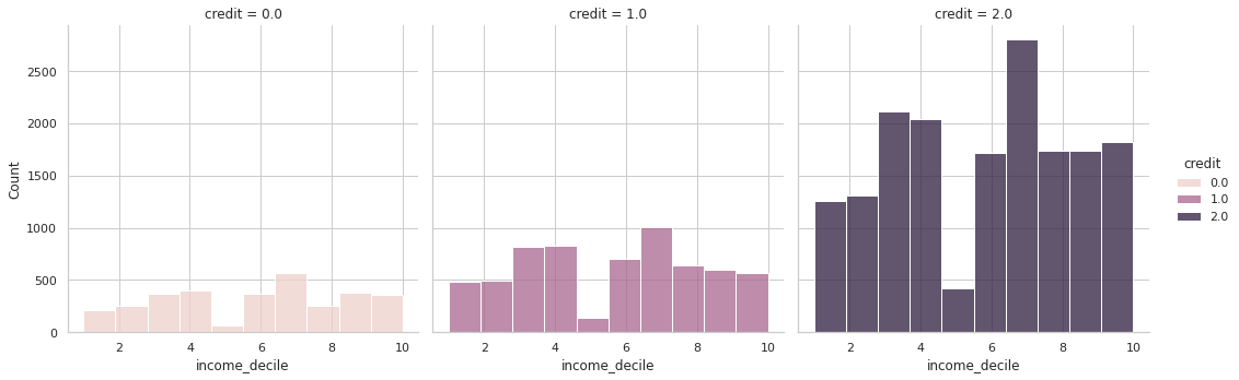
- 현재 4, 5, 10분위에 따라 나누어진 신용 등급표에 의하면 어느 특정 분위수의 그룹이 상대적으로 높게 평가되거나 하진 않는다.
- 수입에 따른 신용등급은 의미가 없을 수도 있다.
6.3 근무 연수에 따른 신용등급
# 근무 연수에 대한 정보
train['worked_year'].describe()
## -1은 무직자를 말한다.
count    26457.000000
mean         5.441736
std          6.581967
min         -1.000000
25%          1.000000
50%          4.000000
75%          8.000000
max         43.000000
Name: worked_year, dtype: float64
creditZero = train[train['credit']==0]
creditOne = train[train['credit']==1]
creditTwo = train[train['credit']==2]plt.figure(figsize=(25, 8))
# 근무 연수에 따른 신용 등급 0의 인원수
plt.subplot(1, 3, 1)
creditZeroPlot = sns.histplot(x='worked_year', hue='credit', bins=43, data=creditZero)
creditZeroPlot.set_xlabel('Worked Years', fontsize=13)
creditZeroPlot.set_ylabel('Number of People', fontsize=13)
creditZeroPlot.set_title("Credit 0's Number of People by Worked Years", fontsize=16)
# 근무 연수에 따른 신용 등급 1의 인원수
plt.subplot(1, 3, 2)
creditOnePlot = sns.histplot(x='worked_year', hue='credit', bins=43, data=creditOne)
creditOnePlot.set_xlabel('Worked Years', fontsize=13)
creditOnePlot.set_ylabel('Number of People', fontsize=13)
creditOnePlot.set_title("Credit 1's Number of People by Worked Years", fontsize=16)
# 근무 연수에 따른 신용 등급 1의 인원수
plt.subplot(1, 3, 3)
creditTwoPlot = sns.histplot(x='worked_year', hue='credit', bins=43, data=creditTwo)
creditTwoPlot.set_xlabel('Worked Years', fontsize=13)
creditTwoPlot.set_ylabel('Number of People', fontsize=13)
creditTwoPlot.set_title("Credit 2's Number of People by Worked Years", fontsize=16)
plt.show()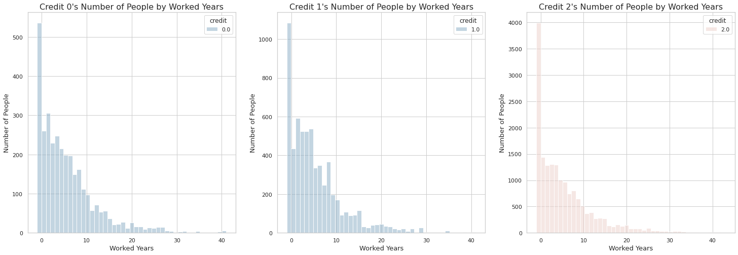
- 전체적인 트랜드를 봤을 때 근무 연수가 올라간다 하여 신용등급이 올라가지는 않는 것으로 보인다.
- 위에서 본 연령별 신용카드 사용자를 보면 50대와 60대의 경우 다른 연령에 비해 사용자가 적다.
- 따라서 근무연수가 올라갈 수록 전체적인 신용등급에 따른 인원이 적은 것으로 보인다.
- 흥미로운점은 무직자가(-1) 신용등급 0에 가장 많다는 것이다.
따라서 근무 연수와 상관없이 신용등급이 결정될 수 있다는 가정이 생긴다.
6.4.1 성별과 근무연수에 따른 신용등급
# 성별에 따른 신용등급 0의 인원수
plt.figure(figsize=(12,7))
genderCreditZero = sns.histplot(x='worked_year', hue='gender', multiple='stack', bins=45, data=creditZero)

genderCreditZero.set_xlabel('Worked Years', fontsize=13)
genderCreditZero.set_ylabel('Number of People', fontsize=13)
genderCreditZero.set_title("Credit 0's Number of Men and Women by Worked Years", fontsize=16)

plt.show()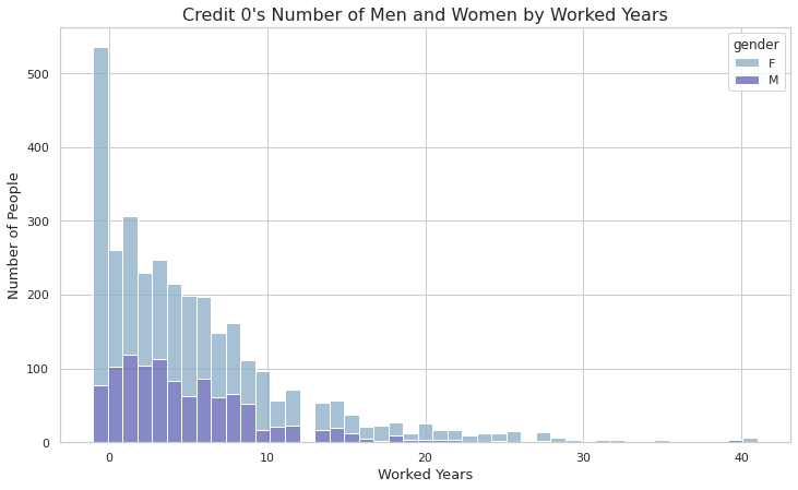
- 신용등급 0 에 대해서 여성의 경우 근무를 하지 않는 그룹이 가장 많은 비중을 차지하고 있다.
# 성별에 따른 신용등급 1의 인원수
plt.figure(figsize=(12,7))
genderCreditOne = sns.histplot(x='worked_year', hue='gender', multiple='stack', bins=45, data=creditOne)

genderCreditOne.set_xlabel('Worked Years', fontsize=13)
genderCreditOne.set_ylabel('Number of People', fontsize=13)
genderCreditOne.set_title("Credit 1's Number of Men and Women by Worked Years", fontsize=16)

plt.show()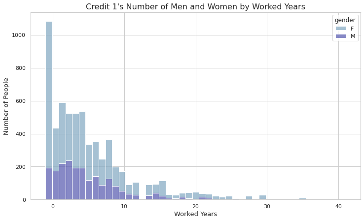
- 신용 등급 1에 대해서도 근무를 하지 않는 여성들이 가장많은 비중을 차지하고 있다.
# 성별에 따른 신용등급 2의 인원수
plt.figure(figsize=(12,7))
genderCreditTwo = sns.histplot(x='worked_year', hue='gender', multiple='stack', bins=45, data=creditTwo)

genderCreditTwo.set_xlabel('Worked Years', fontsize=13)
genderCreditTwo.set_ylabel('Number of People', fontsize=13)
genderCreditTwo.set_title("Credit 2's Number of Men and Women by Worked Years", fontsize=16)

plt.show()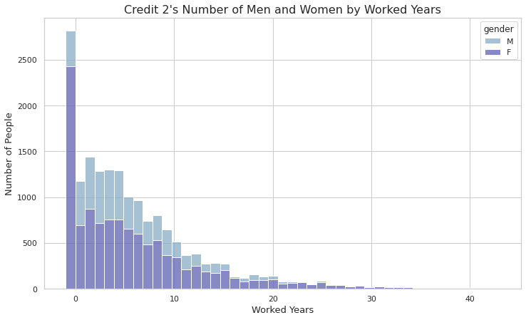
- 신용 등급 2에서는 대부분이 남자가 차지하고 있고 근무연수가 늘어날 수록 비중이 줄어드는 현상이 보인다.
6.4 직업 유형(occpy_type)에 따른 신용등급
- 현재 occyp_type에는 8,171개(31%정도)의 결측치가 존재한다.
- 일한 경력이 없을 경우 직업이 빈칸일 것으로 추측된다.
- 연금 수령자들 또한 직업이 빈칸일 것으로 추측된다.
- 결측치의 비중이 크고 변수에 level이 높아서 drop하는 것이 좋을 수도 있다.
train[train['worked_year']==-1].info()
<class 'pandas.core.frame.DataFrame'>
Int64Index: 4438 entries, 14 to 26443
Data columns (total 22 columns):
 #   Column           Non-Null Count  Dtype
---  ------           --------------  -----
 0   gender           4438 non-null   object
 1   car              4438 non-null   object
 2   reality          4438 non-null   object
 3   child_num        4438 non-null   int64
 4   income_total     4438 non-null   float64
 5   income_type      4438 non-null   object
 6   edu_type         4438 non-null   object
 7   family_type      4438 non-null   object
 8   house_type       4438 non-null   object
 9   DAYS_BIRTH       4438 non-null   int64
 10  DAYS_EMPLOYED    4438 non-null   int64
 11  occyp_type       0 non-null      object
 12  family_size      4438 non-null   float64
 13  begin_month      4438 non-null   float64
 14  credit           4438 non-null   float64
 15  income_quartile  4438 non-null   float64
 16  income_quintile  4438 non-null   float64
 17  income_decile    4438 non-null   float64
 18  age              4438 non-null   int64
 19  age_group        4438 non-null   object
 20  used_years       4438 non-null   int64
 21  worked_year      4438 non-null   int64
dtypes: float64(7), int64(6), object(9)
memory usage: 797.5+ KB- 일한 경력이 없는 4438명의 경우 occyp_type이 Null값으로 되어 있다.
train[train['income_type']=='Pensioner'].info()
<class 'pandas.core.frame.DataFrame'>
Int64Index: 4449 entries, 14 to 26443
Data columns (total 22 columns):
 #   Column           Non-Null Count  Dtype
---  ------           --------------  -----
 0   gender           4449 non-null   object
 1   car              4449 non-null   object
 2   reality          4449 non-null   object
 3   child_num        4449 non-null   int64
 4   income_total     4449 non-null   float64
 5   income_type      4449 non-null   object
 6   edu_type         4449 non-null   object
 7   family_type      4449 non-null   object
 8   house_type       4449 non-null   object
 9   DAYS_BIRTH       4449 non-null   int64
 10  DAYS_EMPLOYED    4449 non-null   int64
 11  occyp_type       9 non-null      object
 12  family_size      4449 non-null   float64
 13  begin_month      4449 non-null   float64
 14  credit           4449 non-null   float64
 15  income_quartile  4449 non-null   float64
 16  income_quintile  4449 non-null   float64
 17  income_decile    4449 non-null   float64
 18  age              4449 non-null   int64
 19  age_group        4449 non-null   object
 20  used_years       4449 non-null   int64
 21  worked_year      4449 non-null   int64
dtypes: float64(7), int64(6), object(9)
memory usage: 799.4+ KB- 9명을 제외한 나머지 4,440명의 경우 직업이 Null값이다.
train[(train['worked_year']==-1)&(train['income_type']=='Pensioner')].info()
<class 'pandas.core.frame.DataFrame'>
Int64Index: 4438 entries, 14 to 26443
Data columns (total 22 columns):
 #   Column           Non-Null Count  Dtype
---  ------           --------------  -----
 0   gender           4438 non-null   object
 1   car              4438 non-null   object
 2   reality          4438 non-null   object
 3   child_num        4438 non-null   int64
 4   income_total     4438 non-null   float64
 5   income_type      4438 non-null   object
 6   edu_type         4438 non-null   object
 7   family_type      4438 non-null   object
 8   house_type       4438 non-null   object
 9   DAYS_BIRTH       4438 non-null   int64
 10  DAYS_EMPLOYED    4438 non-null   int64
 11  occyp_type       0 non-null      object
 12  family_size      4438 non-null   float64
 13  begin_month      4438 non-null   float64
 14  credit           4438 non-null   float64
 15  income_quartile  4438 non-null   float64
 16  income_quintile  4438 non-null   float64
 17  income_decile    4438 non-null   float64
 18  age              4438 non-null   int64
 19  age_group        4438 non-null   object
 20  used_years       4438 non-null   int64
 21  worked_year      4438 non-null   int64
dtypes: float64(7), int64(6), object(9)
memory usage: 797.5+ KB
결측치 처리
- 근무 경험이 없고 연금 수령자인 사람들에 대해서 Unempolyed라는 level로 지정해주자.
- 나머지 값들에 대해선 iterative imputation으로 결측치 처리를 진행하자.
# 무직자와 연금수령자 중 무직자에 대해 Unempolyed 지정
train['occyp_type'][(train.worked_year==-1)&(train.income_type=='Pensioner')] = 'Unempolyed'
train['occyp_type'][train.worked_year==-1] = 'Unempolyed'
train.info()
<class 'pandas.core.frame.DataFrame'>
RangeIndex: 26457 entries, 0 to 26456
Data columns (total 22 columns):
# Column Non-Null Count Dtype
--- ------ -------------- -----
0 gender 26457 non-null object
1 car 26457 non-null object
2 reality 26457 non-null object
3 child_num 26457 non-null int64
4 income_total 26457 non-null float64
5 income_type 26457 non-null object
6 edu_type 26457 non-null object
7 family_type 26457 non-null object
8 house_type 26457 non-null object
9 DAYS_BIRTH 26457 non-null int64
10 DAYS_EMPLOYED 26457 non-null int64
11 occyp_type 22724 non-null object
12 family_size 26457 non-null float64
13 begin_month 26457 non-null float64
14 credit 26457 non-null float64
15 income_quartile 26457 non-null float64
16 income_quintile 26457 non-null float64
17 income_decile 26457 non-null float64
18 age 26457 non-null int64
19 age_group 26457 non-null object
20 used_years 26457 non-null int64
21 worked_year 26457 non-null int64
dtypes: float64(7), int64(6), object(9)
memory usage: 4.4+ MB- 우선 나머지 3733개의 값에 대해선 drop하고 값을 보자
train.dropna(axis=0, inplace=True)
train.info()
<class 'pandas.core.frame.DataFrame'>
Int64Index: 22724 entries, 1 to 26456
Data columns (total 22 columns):
 #   Column           Non-Null Count  Dtype
---  ------           --------------  -----
 0   gender           22724 non-null  object
 1   car              22724 non-null  object
 2   reality          22724 non-null  object
 3   child_num        22724 non-null  int64
 4   income_total     22724 non-null  float64
 5   income_type      22724 non-null  object
 6   edu_type         22724 non-null  object
 7   family_type      22724 non-null  object
 8   house_type       22724 non-null  object
 9   DAYS_BIRTH       22724 non-null  int64
 10  DAYS_EMPLOYED    22724 non-null  int64
 11  occyp_type       22724 non-null  object
 12  family_size      22724 non-null  float64
 13  begin_month      22724 non-null  float64
 14  credit           22724 non-null  float64
 15  income_quartile  22724 non-null  float64
 16  income_quintile  22724 non-null  float64
 17  income_decile    22724 non-null  float64
 18  age              22724 non-null  int64
 19  age_group        22724 non-null  object
 20  used_years       22724 non-null  int64
 21  worked_year      22724 non-null  int64
dtypes: float64(7), int64(6), object(9)
memory usage: 4.0+ MB
# credit값을 object로 치환
train['credit'] = train['credit'].astype('object')
# occyp_type에 따른 신용등급
plt.figure(figsize=(12,7))
occypPlot = sns.histplot(x='occyp_type', hue='credit', multiple='stack', bins=19, data=train)
plt.xticks(rotation = 90)
occypPlot.set_xlabel('Occyp Type', fontsize=13)
occypPlot.set_ylabel('Number of People', fontsize=13)
occypPlot.set_title("Credit Rank Number of People by Occpy Type", fontsize=16)
plt.show()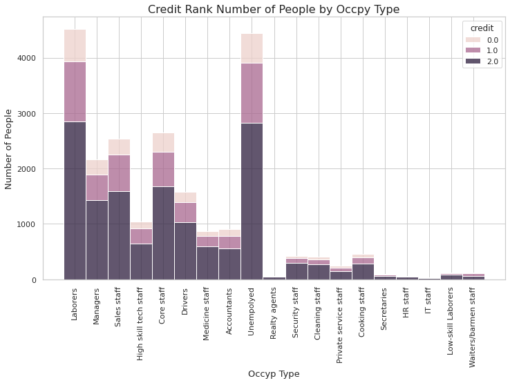
- 현재 직업군에선 'Laboers', 'Managers', 'Sales staff', 'High skill tech staff', 'Core staff', 'Drivers', 'Medicine staff', 'Accountants', 'Unempolyed'가 해석에 있어 의미있는 직업군으로 보인다.
pd.crosstab(train['occyp_type'], train['credit'], normalize='index')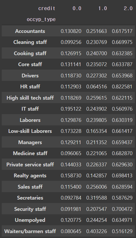
- 현재 체이블에서 보여지는 값으론 사이즈는 작지만 'IT staff'와 'Low-skill Laborers'가 높은 신용등급 0에서의 비율이 가장 높다.