[Tensorflow] Gradient Tape

tf.GradientTape()

forward-propagation 에서 일어나는 연산들을 기억해뒀다가 back-propagation 이 일어날 때 도움을 주는 역할이다.

back-propagation 을 하기 위해서는 forward-propagation에서 사용한 값들이 저장되어 있을 필요가 있다. GradientTap은 forward-propagation 해당 연산 과정에서의 기록을 말한다.

모델에서 뿐 만아니라 prediection이 나오는 부분과 Loss가 나오는 부분 전부가 gradient, 즉 forward-propagation 연산 값들을 저장해야 할 필요가 있다.

t1 = tf.Variable([1, 2, 3], dtype = tf.float32) 
t2 = tf.Variable([10, 20, 30], dtype = tf.float32)

# forward-propagation
with tf.GradientTape() as tape: # tape이라는 이름으로 불러준다.
	t3 = t1 * t2

print(t1.numpy())
print(t2.numpy())
print(t3.numpy())

# 핵심음 Gradient를 바로 받아올 수 있다. 
# 다음은 t3에 대하여 t1과 t2로 편미분 값을 가져온다는 의미이다.
# 최종적으로 Loss L에 대하여 W와 b로 편미분 값을 구할 수 있다.
gradients = tape.gradient(t3, [t1, t2])
print(type(gradients))

print('d_t1', gradients[0])
print('d_t2', gradients[1])

t1 = tf.Variable([1, 2, 3], dtype = tf.float32) 
t2 = tf.Variable([10, 20, 30], dtype = tf.float32)

# forward-propagation
with tf.GradientTape() as tape: # tape이라는 이름으로 불러준다.
	t3 = t1 * t2
	t4 = t3 + t2

gradients = tape.gradient(t4, [t1, t2, t3])
print(type(gradients))

print('d_t1', gradients[0]) 
print('d_t2', gradients[1]) # t2는 t3에 대한 편미분 [1, 2, 3]과 더해진 [1, 1, 1]과 더해 [2, 3, 4]가 된다.
print('d_t3', gradients[2]) # t3는 t4를 만드는데 더하기만 되었기 때문에 편미분의 값이 [1, 1, 1]이 된다.

추가 중요 개념

constant 는 input이 되는 것으로 update되지 않기 때문에 back-propagation 에 필요가 없다.

t1 = tf.constant([1, 2, 3], dtype = tf.float32) 
t2 = tf.Variable([10, 20, 30], dtype = tf.float32)

# forward-propagation
with tf.GradientTape() as tape: 
	t3 = t1 * t2
	t4 = t3 + t2

gradients = tape.gradient(t3, [t1, t2])
print(type(gradients))

print('d_t1', gradients[0]) # None이 출력된다.
print('d_t2', gradients[1])

linear regression

X_data = tf.random.normal(shape = (1000,), dtype = tf.float32)
y_data = 3 * x_data + 1 # noise 적용하지 않음

print(x_data.dtype, y_data.dtype)

# singal linear regression
# variable 이 2개가 필요하다.
w = tf.Variable(-1.) # initalize를 -1로 해준다.
b = tf.Variable(-1.)

laerning_rate = 0.01
EPOCHS = 10

w_trace, b_trace = [], [] # w, b의 업데이트 과정을 확인하기 위해

# 딥러닝
for epoch in range(EPOCHS):
	for x, y in zip(x_data, y_data): # zip은 x_data나 y_data를 하나씩 뽑아오는 것
		# forward-propagation
		with tf.GradientTap() as tape:
			prediction = wx + b
			loss = (prediction - y) ** 2 # 제곱

		gradients = tape.gradient(loss, [w, b])

		w_trace.append(w.numpy())
		b_trace.append(b.numpy())

		# Stochastic Gradient Descent
		# 확률적 경사하강법
		w = tf.Variable(w - laerning_rate * gradients[0]) # laerning_rate * gradients[1]는 constant 텐서이기 때문에 variable로 변경해준다.
		b = tf.Variable(b - laerning_rate * gradients[1])

fig, ax = plt.subplots(figsize = (20, 10))

ax.plot(w_trace, label='weight')
ax.plot(b_trace, label='bias')

ax.tick_params(labelsize=20)
ax.legend(fontsize=30)
ax.grid()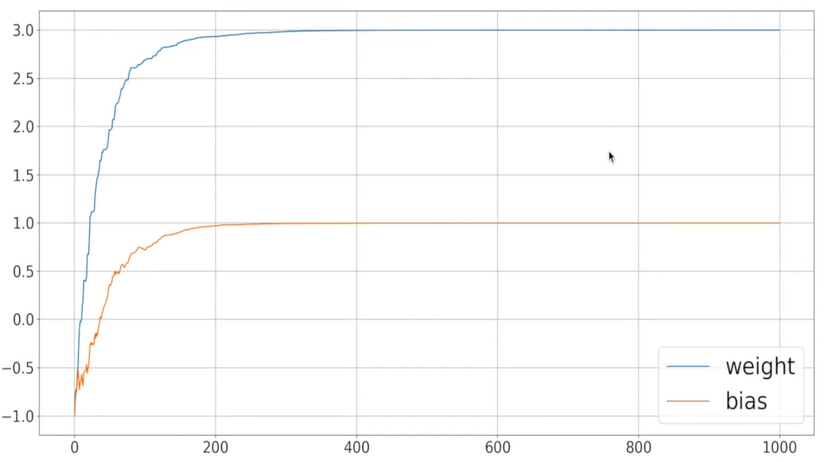

처음 설정한 initalize한 -1에서 weight는 3까지, bias는 1까지 이동한 것을 볼 수 있다.

with tf.GradientTap() as tape:
			prediction = model
			loss = lossobject

다음과 같은 형태로 forward-propagation를 작성해준다.