[Tensorflow] 모델 구현하기 1

데이터셋을

러닝 모델에 넣어주고

foward propagation을 통해서

Loss를 계산해주고

optim을 통해서 모델을 학습해준다.

Model 만들기

• sequential - 기본적인 것들, 자율성이 떨어짐
• functional -
• model subclassing - 자율성이 있음

---

keras 를 이용한 sequential 모델 만들기

import tensorflow as tf

x_train = tf.random.normal(shape=(1000, ), dtype=tf.float32)
y_train = 3 * x_train + 1 + 0.2 * tf.random.normal(shape=(1000,), dtype=tf.float32)

# 데이터 시각화 
fig ,ax = plt.subplots(figsize=(10, 10))
ax.scatter(x_train.numpy(),
           y_train.numpy())
ax.tick_params(labelsize=20)
ax.grid()

기존의 y = 3 x + 1 예측에 `0.2 tf.random.normal(shape=(1000,), dtype=tf.float32)` 를 추가해 줌으로써 모델의 noise 를 추가해 준다.

그래프 출력을 위해서는 console창에 %matplotlib qt 를 출력해 준다.

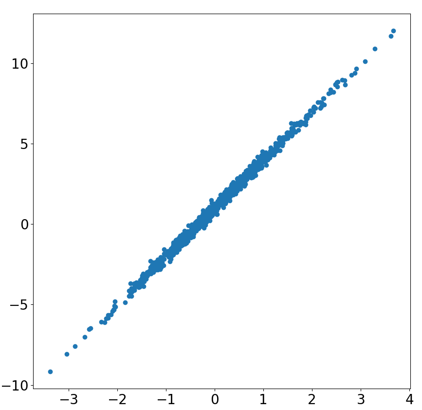
위와 같은 Linear 한 prediction 예측값을 만들기 위해서(목적)

y = wx + b or y = xw + b 일떄 하나의 뉴런이 필요한데

Artificial Neuron = Affine Function + Activation Function

Artificial Neuron 는 주어진 입력에서 특정 패턴을 추출해내는 함수를 의미한다.

Affine Function 은 Weight와 Bias를 학습하는 과정

Activation Function 은 Sigmoid Function, Tanh Function, ReLU Function 등

ŷ = wx + b 가 prediction 이라고 한다면, Loss 를 계산할 때 L = ( y - ŷ )^2 로 MSE를 적용해서 만들어 낸다. 이는 activation function 이 필요 없는 것이며 Linear 한 것임을 알 수 있다.

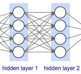
위와 같은 그림은 Dense한 layer로 하나의 layer의 노드값이 다음 layers에 fully connected 하게 연결된다. tf.keras.layers.Dense(units = 1, activation = 'linear') 로 Dense layer를 만들 수 있다. units은 뉴런의 개수로 Dense layer하나의 계층 안에 들어있는 뉴런들 전체가 activation function 을 가진다.

# keras를 이용한 sequential 모델 만들기

model = tf.keras.models.Sequential([
    tf.keras.layers.Dense(units=1,
                          activation='linear')

    ])

model.compile(loss='mean_squared_error', optimizer='SGD')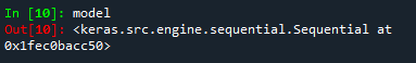

모델이 생성된 것을 확인할 수 있다. 모델을 내부의 아키텍쳐를 구성해주고 컴파일을 진행하면 학습 준비가 완료된다. model에 Loss, optim 이라는 오브젝트를 달아주어 foward와 back를 모두 한번에 연산을 할 수 있다.

model.fit(x_train, y_train, epochs=50, verbose=1)
model.evaluate(x_test, y_test, verbose=2)

학습하는 단계는 다음과 같다. 모델선언, Loss, optimizer, 컴파일, 러닝, 평가

---

subclass 로 만드는 모델

tf.keras.model. 을 class 에 상속 시켜줌으로써 내부에서 특징들을 사용한다. LinearPredictor() 를 호출하면 init 를 자동으로 실행시키고, 상속 받은 것들을 실행시키고, Dense layer를 하나 가지고 있게 된다. call 함수를 통해서 forward propagtion 이 어떻게 일어나는지 작성한다.

# 아래 3줄은 고정 format
# subclass를 이용한 모델 만들기

from termcolor import colored

class LinearPredictor(tf.keras.Model):
    def __init__(self):
        super(LinearPredictor, self).__init__()

        self.dl = tf.keras.layers.Dense(units=1, activation='linear')
    def call(self, x):
        x = self.dl(x)
        return x

keras의 sequential 모델로는 순차적이지 않고 jump 과정을 적용하기 어렵다. 그러므로 어떻게 forward propagtion 이 진행될지 설명이 필요하다.

간단한 모델의 경우 sequential 하기 때문에 keras 모델을 사용하는 것이 적합하고, forward propagtion 이 어떻게 일어날지 세부적으로 정해줄 수 있기 위해서는 subclass 를 사용한다.

EPOCHS = 10
LR = 0.01

## instantiation learning object
model = LinearPredictor()
loss_object = tf.keras.losses.MeanSquaredError() # complie 
optimizer = tf.keras.optimizers.SGD(learning_rate=LR) # optimizer

모델을 만들고 complie 과 optimizer를 해주는 것이 아니라 오브젝트를 따로 만들어 준다. 모델을 인스턴스화해준다.

batch 로 불러오지 않고 x_train, y_train 를 하나씩 받아온다. model(x) 는 LinearPredictor 를 인스턴스화한 것으로 call() 함수를 불러온다. Dense layer 하나를 통과해서 x 로 덮어씌우고 return 해준다.

## learning
for epoch in range(EPOCHS):
    for x, y in zip(x_train, y_train):
        x = tf.reshape(x, (1,1))

        ### forward propogation
        with tf.GradientTape() as tape:
            predictions = model(x)
            loss = loss_object(y, predictions)

        ### backward propogation
        gradients = tape.gradient(loss, model.trainable_variables)

        ### parameter update
        optimizer.apply_gradients(zip(gradients, model.trainable_variables))
    
    print(colored('Epoch: ', 'red', 'on_white'), epoch+1)
    template = 'train loss : {} \n'
    print(template.format(loss))

이전 시간에서의 모델과 Loss 까지의 일어나는 부분까지 tape로 저장해둔다 를 forward propagation으로 구현해준다.

이후 tape에 저장해둔 값을 이용해 backward propagation 과정으로 gradient를 구한다. model.trainable_variables 에는 units 개수만큼의 W와 bias 벡터가 담겨있다.

optimizer를 통해 parameter의 값을 update해준다.

---

정리

simple linear regression

• keras를 사용한 경우 모델을 단순하게 sequential 하게 만들어주고 compile를 해주면 loss 와 object가 만들어진다. 이후 fit 하면 학습 완료
  

model = tf.keras.models.Sequential([
    tf.keras.layers.Dense(units=1,
                          activation='linear')

    ])

model.compile(loss='mean_squared_error', optimizer='SGD')

model.fit(x_train, y_train, epochs=50, verbose=1)
model.evaluate(x_test, y_test)

• subclass를 통해 구현 모델을 layer를 구현해주고 어떻게 forward propagation 할지 정의해주고 call를 불러줌으로써 모델을 한번 인스턴스화 해주고 loss와 optimizer 를 원하는 것으로 가져와준다. epoch을 돌리고 하나씩 불러와서 forward propagation 에서의 연산들을 tape에 기록해 주었다가 back propogation 에서 gradient를 구하고 , parameter update를 하면서 학습을 진행한다.
  

from termcolor import colored

class LinearPredictor(tf.keras.Model):
    def __init__(self):
        super(LinearPredictor, self).__init__()
        self.dl = tf.keras.layers.Dense(units=1, activation='linear')
    def call(self, x):
        x = self.dl(x)
        return x
    
EPOCHS = 10
LR = 0.01

## instantiation learning object
model = LinearPredictor()
loss_object = tf.keras.losses.MeanSquaredError()
optimizer = tf.keras.optimizers.SGD(learning_rate=LR)

## learning
for epoch in range(EPOCHS):
    for x, y in zip(x_train, y_train):
        x = tf.reshape(x, (1,1))
        ### forward propogation
        with tf.GradientTape() as tape:
            predictions = model(x)
            loss = loss_object(y, predictions)
        ### backward propogation
        gradients = tape.gradient(loss, model.trainable_variables)
        ### parameter update
        optimizer.apply_gradients(zip(gradients, model.trainable_variables))
    
    print(colored('Epoch: ', 'red', 'on_white'), epoch+1)
    template = 'train loss : {} \n'
    print(template.format(loss))