[Tensorflow] 모델 구현하기 2

지난 시간은 simple linear regression 학습하였다.

이번 시간은 classification 을 구현해보도록 하자!

import tensorflow as tf
import numpy as np
import matplotlib.pyplot as plt

n_sample = 100
x_train = np.random.normal(0,1,size=(n_sample,1))
y_train = (x_train >= 0).astype(np.float32)
print(y_train)

랜덤한 값으로 100개를 구현했을 때 0보다 크면 true로 작으면 false를 내보낸다. 뒤에 astype() 함수를 사용해서 데이터의 타입을 변경해 줄 수 있다.

# 데이터 시각화
plt.style.use('seaborn')

n_sample = 100
x_train = np.random.normal(0,1,size=(n_sample,1))
y_train = (x_train >= 0).astype(np.float32)
print(y_train)

fig, ax = plt.subplots(figsize=(20,10))
ax.scatter(x_train, y_train)
ax.tick_params(labelsize=20)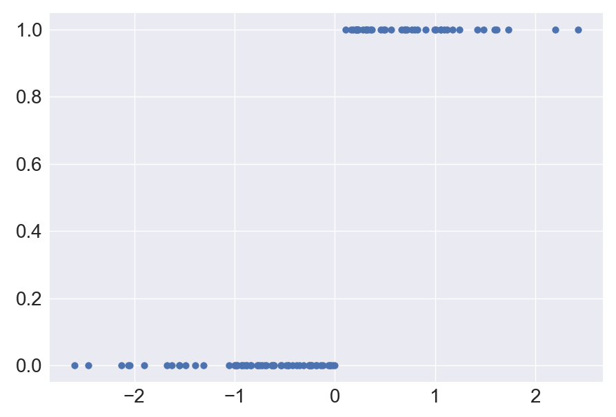

해당 데이터를 binary classification 해보도록 한다. noise를 적용하지 않았음. 0보다 크면 합격, 0보다 작으면 불합격으로 분류한다. 해당 데이터는 타입이 float64임으로 .astype(np.float32)를 추가해 float32로 선언해주도록 한다.

classification model를 만들어보자

# classification model
class classifier(tf.keras.Model):
    def __init__(self):
        super(classifier, self).__init__()
        
        self.dl = tf.keras.layers.Dense(units=1, activation='sigmoid')
        
    def call(self, x):
        predictions = self.dl(x)
        return predictions

simple regression model과 동일하게 처음 3줄은 그대로 작성해준다. Dense layer에는 뉴런이 하나 들어 있고, 해당 모델은 binary classification 모델이기 때문에 activation function을 sigmoid 함수로 지정해 준다.

## hyper parameter
EPOCHS = 10
LR = 0.01

## instantiation learning object
model = classifier()
loss_object = tf.keras.losses.BinaryCrossentropy()
optimizer = tf.keras.SGD(learning_rate=LR)

모델은 인스턴스화 해준다. 이전 시간에서는 loss 함수를 Mean_squared_error를 사용하였지만, 이번 시간은 binary classification 이기 때문에 binarycrossentropy 를 사용한다. optimizer는 동일하게 SGD 를 사용한다.

# learning
for epoch in range(EPOCHS):
    for x, y in zip(x_train, y_train):
        x = tf.reshape(x, (1,1))
        # print(x.shape, y.shape) 
        
        with tf.GradientTape() as tape:
            predictions = model(x)
            loss = loss_object(y, predictions)
            
        gradients = tape.gradient(loss, model.trainable_variables)
        optimizer.apply_gradients(zip(model, model.trainable_variables))
        
    print(colored('Epoch: ', 'cyan', 'on_white'), epoch+1)
    template = 'train loss : {} \n'
    
    print(template.format(loss))

optimizer과정에서 gradient와 모델이 가진 trainable paramter에 적용한다.

위의 모델은 하나의 iteration이 진행되어 loss를 계산한다. 마지막 loss에 대한 결과를 출력하기 때문에 부정확하다. 데이터 셋 전체의 loss들을 누적해서 평균값을 구해주어야 한다. accurracy 라는 계산을 통해서 평균값을 구해보도록 하자.

loss_metric = tf.keras.metrics.Mean()
acc_metric = tf.keras.metrics.CategoricalAccuracy()

Mean() 함수는 하나의 전체 데이터셋에 대한 Loss의 평균값을 내보내준다. CategoricalAccuracy() 는 y 와 예측값 y 의 차이를 loss로 정의할 때, 값이 맞았는지 맞지 않았는지의 비율 값을 내보낸다.

for x, y in zip(x_train, y_train): 함수의 내부가 하나의 iteration 이 된다.

ds_loss = loss_metric.result()
ds_acc = acc_metric.result()
    
loss_metric.reset_states()
acc_metric.reset_states()

전체 epoch 이 끝났을 때 result() 를 통해 출력하며, 반드시 reset_states() 를 해주어야 한다.

# classification model
class classifier(tf.keras.Model):
    def __init__(self):
        super(classifier, self).__init__()
        
        self.dl = tf.keras.layers.Dense(units=1, 
                                        activation='sigmoid')
        
    def call(self, x):
        predictions = self.dl(x)
        return predictions

## hyper parameter
EPOCHS = 10
LR = 0.01

## instantiation learning object
model = classifier()
loss_object = tf.keras.losses.BinaryCrossentropy()
optimizer = tf.keras.optimizers.SGD(learning_rate=LR)

loss_metric = tf.keras.metrics.Mean()
acc_metric = tf.keras.metrics.CategoricalAccuracy()

# learning
for epoch in range(EPOCHS):
    for x, y in zip(x_train, y_train):
        x = tf.reshape(x, (1,1))

        # print(x.shape, y.shape) 
        
        with tf.GradientTape() as tape:
            predictions = model(x)
            loss = loss_object(y, predictions)
            
        gradients = tape.gradient(loss, model.trainable_variables)
        optimizer.apply_gradients(zip(gradients, model.trainable_variables))
        
        loss_metric(loss)
        acc_metric(y, predictions)
        
    print(colored('Epoch: ', 'cyan', 'on_white'), epoch + 1)
    template = 'train loss : {.4f} \t Train Accuracy : {:.2f}%'
    
    ds_loss = loss_metric.result()
    ds_acc = acc_metric.result()
    
    print(template.format(ds_loss, ds_acc*100))
    
    loss_metric.reset_states()
    acc_metric.reset_states()

다음 시간에는 2개의 값을 가지는 units =1 은 동일!

input demension, 즉 데이터 셋 내의 피쳐(attribute)의 개수가 2개일 때를 알아보자