로지스틱 회귀

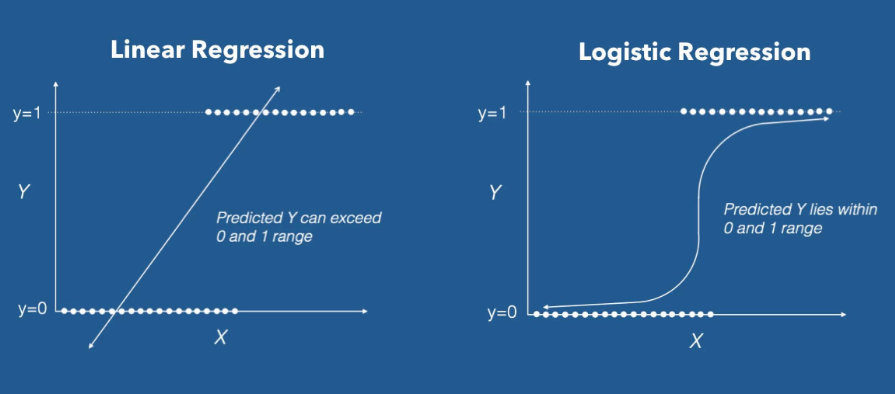
예측해야 하는 데이터가 범주형 자료일 때는 선형 회귀를 쓸 수 없다.
로지스틱 회귀는 종속변수(Y)가 0~1의 값을 가지기 때문에 결과값을 확률로 표현할 수 있다.

오즈 (Odds)

로지스틱 함수를 이해하기 위해서는 Odds 라는 개념을 알아야 한다.

Odds(승산): 임의의 사건 A가 발생하지 않을 확률 대비 일어날 확률의 비율.

$\frac { P(A) }{ P({ A }^{ c }) } =\frac { P(A) }{ 1-P(A) }$

오즈는 0에서 무한의 값을 가진다. P(A)가 성공확률이라고 했을 때, 0일 경우 실패확률은 1이 되어 오즈는 0이 될 것이고, 1일 경우 무한이 될 것이다.

로짓 변환

흔히 아는 확률 (Probability. $\frac {성공횟수}{전체 시도 횟수}$ ) 을 써서 회귀식을 만들면 다음과 같다.

$P(Y=1\ |\ \mathbf{x} ) \ne \beta_0 + \beta_1 x_1 + \beta_2 x_2 + ... + \beta_n x_n$

이 수식의 문제는 좌변은 확률이기 때문에 0~1의 값을 가지지만, 우변은 음의 무한부터 양의 무한이라는 것이다.

그래서 Odds ratio (오즈비)로 바꿔주었더니

참고로 오즈비 란 Y=1 일 때 오즈를 Y=0 일 때의 오즈로 나눈 비율이다.

어쨌든 오즈비의 범위도 0에서 무한대이기 때문에 범위가 여전히 안 맞는다.

그래서 로짓 변환 이라는걸 해준다. 좌변에 로그 함수를 씌우는 것. 로짓 변환한 함수는 이렇게 생겼다.

이 P(x)가 바로 로지스틱 함수가 된다.

로지스틱 함수는 '시그모이드 함수'라고도 부르는데, Neural Network 에서 쓰이는 그 시그모이드 함수가 맞다.

📘 Kaggle

데이터 설명

심장병 예측 태스크
향후 10년간 '관상동맥질환(Coronary Heart Disease)' 발병 가능성 예측
15개의 변수

Each attribute is a potential risk factor. There are both demographic, behavioural and medical risk factors.

• Demographic
  sex: male or female;(Nominal)
  age: age of the patient;(Continuous - Although the recorded ages have been truncated to whole numbers, the concept of age is continuous)

• Behavioural
  currentSmoker: whether or not the patient is a current smoker (Nominal)
  cigsPerDay: the number of cigarettes that the person smoked on average in one day.(can be considered continuous as one can have any number of cigarretts, even half a cigarette.)

• Medical( history):
  BPMeds: whether or not the patient was on blood pressure medication (Nominal)
  prevalentStroke: whether or not the patient had previously had a stroke (Nominal)
  prevalentHyp: whether or not the patient was hypertensive (Nominal)
  diabetes: whether or not the patient had diabetes (Nominal)

• Medical(current):
  totChol: total cholesterol level (Continuous)
  sysBP: systolic blood pressure (Continuous)
  diaBP: diastolic blood pressure (Continuous)
  BMI: Body Mass Index (Continuous)
  heartRate: heart rate (Continuous - In medical research, variables such as heart rate though in fact discrete, yet are considered continuous because of large number of possible values.)
  glucose: glucose level (Continuous)

Predict variable (desired target):

10 year risk of coronary heart disease CHD (binary: “1”, means “Yes”, “0” means “No”)
In [3]:

NaN값은 모두 제거하였다.

EDA

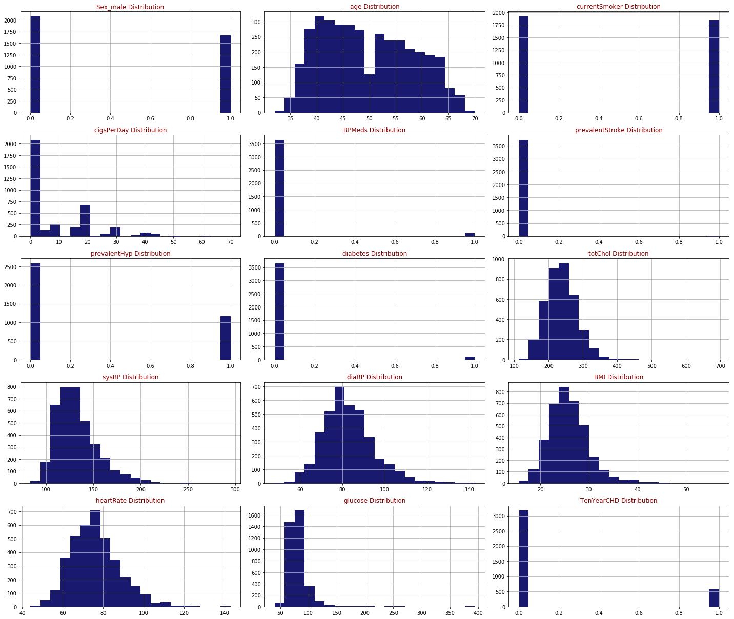
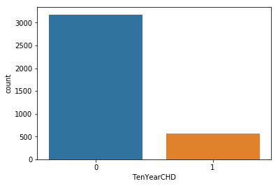
심장병의 위험이 없는 환자가 3179명, 심장병 위험이 있는 환자가 572명이었다.

로지스틱 회귀 모델

add_constant

from statsmodels.tools import add_constant as add_constant
heart_df_constant = add_constant(heart_df)
heart_df_constant.head()

add_constant는 상수항을 생성하는 함수로, 선형회귀분석에서는 수식을 간결하게 만들기 위해 상수항을 더하는데 이걸 상수항 결합 (bias augmentation) 이라고 부른다.

유의미한 변수만 남기기

st.chisqprob = lambda chisq, df: st.chi2.sf(chisq, df)
cols=heart_df_constant.columns[:-1]
model=sm.Logit(heart_df.TenYearCHD,heart_df_constant[cols])
result=model.fit()
result.summary()

Optimization terminated successfully.
Current function value: 0.377036
Iterations 7

alpha(0.05)보다 큰 P-value는 통계적으로 유의미하지 않기 때문에 backward elimination 방법으로 0.05보다 작은 P-value를 가진 피쳐들만 남을때까지 카이제곱 검정을 반복한다.

여기서 Logit은 logit model을 의미하는데, 종속변수와 독립변수들의 관계를 확률적으로 계산하는 모델이라고 한다.

def back_feature_elem (data_frame,dep_var,col_list):
    """ Takes in the dataframe, the dependent variable and a list of column names, runs the regression repeatedly eleminating feature with the highest
    P-value above alpha one at a time and returns the regression summary with all p-values below alpha"""

    while len(col_list)>0 :
        model=sm.Logit(dep_var,data_frame[col_list])
        result=model.fit(disp=0)
        largest_pvalue=round(result.pvalues,3).nlargest(1)
        if largest_pvalue[0]<(0.05):
            return result
            break
        else:
            col_list=col_list.drop(largest_pvalue.index)

result=back_feature_elem(heart_df_constant,heart_df.TenYearCHD,cols)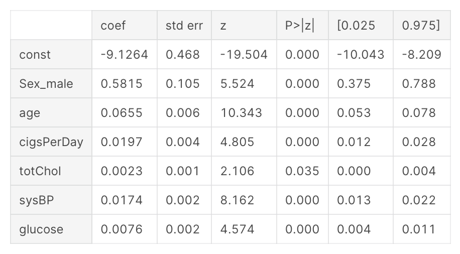

7개의 피쳐들만 남은걸 볼 수 있다.

$logit(p) = log(p/(1-p))=\beta_0 +\beta_1\hspace{.1cm} *\hspace{.2cm} Sexmale\hspace{.2cm}+\beta_2\hspace{.1cm} * \hspace{.1cm}age\hspace{.2cm}+\hspace{.2cm}\beta_3\hspace{.1cm} *\hspace{.1cm} cigsPerDay\hspace{.2cm}+\hspace{.2cm}\beta_4 \hspace{.1cm}*\hspace{.1cm} totChol\hspace{.2cm}+\hspace{.2cm}\beta_5\hspace{.1cm} *\hspace{.1cm} sysBP\hspace{.2cm}+\hspace{.2cm}\beta_6\hspace{.1cm} *\hspace{.1cm} glucose\hspace{.2cm}$

$\beta_0$ 는 상수항이고, 나머지 변수들을 합해서 로지스틱 회귀식을 만들면 이렇게 생겼다.

해석

params = np.exp(result.params)
conf = np.exp(result.conf_int())
conf['OR'] = params
pvalue=round(result.pvalues,3)
conf['pvalue']=pvalue
conf.columns = ['CI 95%(2.5%)', 'CI 95%(97.5%)', 'Odds Ratio','pvalue']
print ((conf))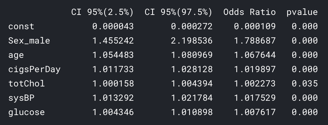

오즈비를 퍼센트로 환산하면 (1-x)*100%를 하면 된다.
즉 오즈비가 1.5면 50%의 증가를 보이는 것.

• 남자가 여자보다 오즈가 78.8% 높았다.
• 나이가 한 살 많을수록 심장병 발병 가능성이 7% 증가했다.
• 담배 한 개비씩 필 때마다 2% 증가했다.
• 콜레스테롤과 글루코스는 오즈에 유의미한 변화를 보이지 않았다.
• 혈압이 높을수록 1.7% 증가를 보였다.

모델 평가

from sklearn.linear_model import LogisticRegression
logreg=LogisticRegression()
logreg.fit(x_train,y_train)
y_pred=logreg.predict(x_test)

Confusion Matrix

sklearn.metrics.accuracy_score(y_test,y_pred)

0.881491344873502

from sklearn.metrics import confusion_matrix
cm=confusion_matrix(y_test,y_pred)
conf_matrix=pd.DataFrame(data=cm,columns=['Predicted:0','Predicted:1'],index=['Actual:0','Actual:1'])
plt.figure(figsize = (8,5))
sn.heatmap(conf_matrix, annot=True,fmt='d',cmap="YlGnBu")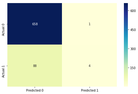

662개(658+4)는 제대로 예측했다.

ROC Curve

from sklearn.metrics import roc_curve
fpr, tpr, thresholds = roc_curve(y_test, y_pred_prob_yes[:,1])
plt.plot(fpr,tpr)
plt.xlim([0.0, 1.0])
plt.ylim([0.0, 1.0])
plt.title('ROC curve for Heart disease classifier')
plt.xlabel('False positive rate (1-Specificity)')
plt.ylabel('True positive rate (Sensitivity)')
plt.grid(True)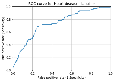

sklearn.metrics.roc_auc_score(y_test,y_pred_prob_yes[:,1])

0.73551824239625252

AUC(ROC 아래 면적)는 0.74 정도가 나왔다. 1에 가까울수록 이상적인데, 이 정도면 괜찮다고 볼 수 있다.

결론

• 예측에 사용한 피쳐는 모두 0.05 이하의 P-value 를 가진 것으로, 심장병 예측에 유의미한 역할을 한다고 볼 수 있다.
• 남자가 여자보다 심장병에 취약한 것으로 보이며, 나이가 많을수록, 흡연 횟수와 혈압이 높을수록 심장병의 가능성이 높았다.
• 콜레스테롤과 글루코스는 큰 영향을 보이지 않았다.
• 모델의 정확도는 0.88로 민감도보다 특이도가 높다.

---

참고

로지스틱 회귀

로지스틱 수식