[핸즈온 ML with Kaggle] 5. Decision Tree: Pruning

김서연·2021년 11월 6일

핸즈온 머신러닝 with Kaggle

목록 보기

4/6

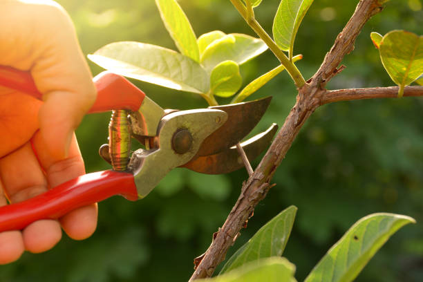
~~싹둑!~~

🌳Pruning 이란?

"Pruning" 은 '가지치기'라는 뜻이다. 머신러닝에서는 Decision Tree 의 가지를 자른다, 즉 모델에 제한을 줘서 오버피팅을 방지하는 기법이다.
Pruning의 종류로는 Pre-pruning 과 Post-Pruning 이 있다.

Pre-Pruning

pre-pruning은 다른 말로 early stopping 이라고도 한다. 말 그대로 학습을 일찍 멈춘다는 뜻. pre-pruning은 모델의 깊이와 가지 개수를 지정하는 hyperparameter 값을 조정해주면 된다.
Grid Search와 같은 하이퍼파라미터 튜닝 기법으로 pre-pruning을 효율적으로 진행할 수 있다.

Post-Pruning

post-pruning은 Decision Tree로 학습을 시킨 후에 가지치기를 하는 방법이다.
가장 많이 쓰이는 방법은 Cost-Complexity Pruning인데, 가장 영향이 작은 '알파'값을 찾아서 그 값을 가진 노드부터 가지치기 한다.

$R(T)$ : 리프 노드의 총 학습 에러
$|T|$ : 리프 노드 개수
$a$ : complexity 파라미터

$R(T)$ 만 줄이려고 한다면 트리의 규모가 커져 (가지 수가 많아짐) 오버피팅이 될 수 있다. $a$ 는 남길 리프 노드 개수를 정하기 때문에 $a$ 를 조절하면서 오버피팅을 방지할 수 있다. $a$ 값이 커질수록 가지치기하는 노드가 많아진다.

sub-tree에 대해서도 $R_a(T_t)$ 값을 구한다.

📘Kaggle

오늘 리뷰할 노트북

Decision Tree model building

clf = tree.DecisionTreeClassifier(random_state=0)
clf.fit(x_train,y_train)
y_train_pred = clf.predict(x_train)
y_test_pred = clf.predict(x_test)

pruning 안 한 accuracy score

Train score 1.0
Test score 0.7631578947368421

train score은 1인데 test score은 0.76밖에 안 된다?! → 오버피팅이군 → 가지치기를 하자!

⏪Pre-Pruning

Parameters:

max_depth: 트리의 깊이
min_sample_split: 분할되기 위해 노드가 가져야 하는 최소 샘플 수
min_samples_leaf: 리프 노드가 가지고 있어야 할 최소 샘플 수

Pruning with Grid Search

파라미터 값을 리스트로 넣어주고, Grid Search로 최적의 파라미터 조합을 찾는 과정

params = {'max_depth': [2,4,6,8,10,12],
         'min_samples_split': [2,3,4],
         'min_samples_leaf': [1,2]}

clf = tree.DecisionTreeClassifier()
gcv = GridSearchCV(estimator=clf,param_grid=params)
gcv.fit(x_train,y_train)

model = gcv.best_estimator_
model.fit(x_train,y_train)
y_train_pred = model.predict(x_train)
y_test_pred = model.predict(x_test)

pre-pruning accuracy score

Train score 0.9647577092511013
Test score 0.7894736842105263

pre-pruning을 했더니 test score가 0.79 정도로 아까(0.76)보다는 미세하게 나아졌다.

⏩Post-Pruning

path = clf.cost_complexity_pruning_path(x_train, y_train)
ccp_alphas, impurities = path.ccp_alphas, path.impurities
print(ccp_alphas)

[0. 0.00469897 0.00565617 0.00630757 0.00660793 0.00660793
0.00704846 0.00739486 0.0076652 0.0077917 0.00783162 0.00792164
0.00802391 0.00926791 0.01082349 0.01151248 0.01566324 0.02484071
0.04195511 0.04299238 0.13943465]

위의 알파들로 학습시켜서 결과를 비교해볼 것이다.

# For each alpha we will append our model to a list
clfs = []
for ccp_alpha in ccp_alphas:
    clf = tree.DecisionTreeClassifier(random_state=0, ccp_alpha=ccp_alpha)
    clf.fit(x_train, y_train)
    clfs.append(clf)

.cost_complexity_pruning_path 메소드는 각 가지치기 과정마다 효과적인 알파값과 불순도를 반환한다고 한다.

# 마지막 트리는 노드 한 개로 이루어져 있어서 그냥 제외했다고 함.
clfs = clfs[:-1]
ccp_alphas = ccp_alphas[:-1]

node_counts = [clf.tree_.node_count for clf in clfs]
depth = [clf.tree_.max_depth for clf in clfs]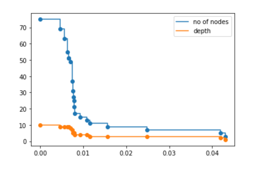

알파의 값이 커짐에 따라 노드의 개수와 트리의 깊이는 줄어든다.

여러 알파로 학습시킨 결과

train_acc = []
test_acc = []
for c in clfs:
    y_train_pred = c.predict(x_train)
    y_test_pred = c.predict(x_test)
    train_acc.append(accuracy_score(y_train_pred,y_train))
    test_acc.append(accuracy_score(y_test_pred,y_test))

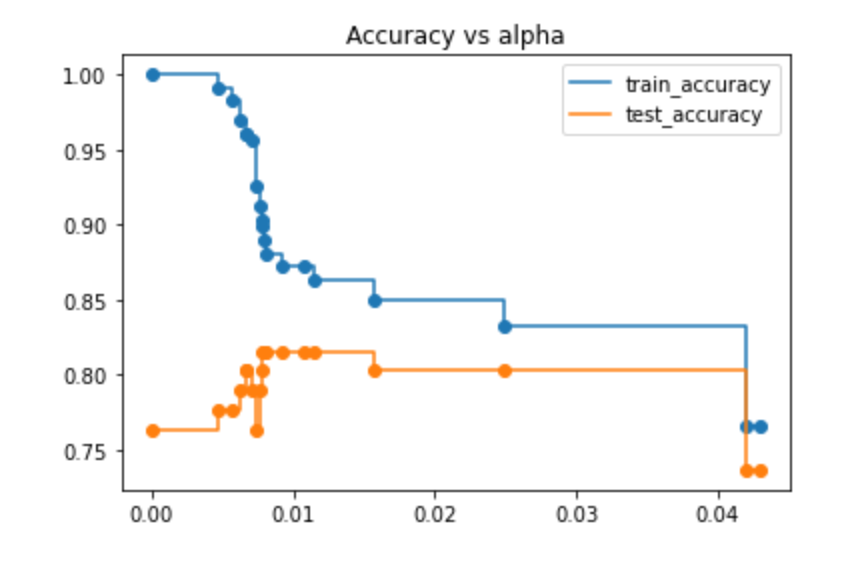
train accuracy와 test accuracy를 비교했을 때 0.02가 제일 차이가 없어보여서 + train accuracy도 크게 낮아지지 않아서 0.020 으로 결정했다.

최적의 알파로 다시 학습

clf_ = tree.DecisionTreeClassifier(random_state=0,ccp_alpha=0.020)
clf_.fit(x_train,y_train)
y_train_pred = clf_.predict(x_train)
y_test_pred = clf_.predict(x_test)