Regression (회귀분석)

Jihwan Oh·2023년 12월 13일

data analysis

목록 보기

5/9

모듈 불러오기

# 데이터 전처리 패키지
import numpy as np #수치해석 패키지로 행렬식 계산할 때 주로 사용됨.
import pandas as pd #데이터를 엑셀과 같은 형태로 보여지도록 만들어주는 패키지

# 회귀모델 구축 및 평가 패키지
import statsmodels
import statsmodels.formula.api as smf
from statsmodels import regression
from scipy import stats

# 데이터 시각화 패키지
import pylab
from matplotlib import font_manager, rc, rcParams
import matplotlib.pyplot as plt

데이터 만들기

height = np.array([181, 161, 170, 160, 158, 168, 162, 179, 183, 178,
                   171, 177, 163, 158, 160, 160, 158, 173, 160, 163,
                   167, 165, 163, 173, 178, 170, 167, 177, 175, 169,
                   152, 158, 160, 160, 159, 180, 169, 162, 178, 173,
                   173, 171, 171, 170, 160, 167, 168, 166, 164, 173,
                   180])
weight = np.array([78, 49, 52, 53, 50, 57, 53, 54, 71, 73,
                   55, 73, 51, 53, 65, 48, 59, 64, 48, 53,
                   78, 45, 56, 70, 68, 59, 55, 64, 59, 55,
                   38, 45, 50, 46, 50, 63, 71, 52, 74, 52,
                   61, 65, 68, 57, 47, 48, 58, 59, 55, 74,
                   74])
test_height = np.array([150.5, 155.5, 160.5, 165.5, 170.5, 175.5, 180.5, 185.5, 190])

DataFrame 패키지

데이터분석 라이브러리.
아래와 같이 행과 열로 이루어진 데이터 객체를 만들수 있음.

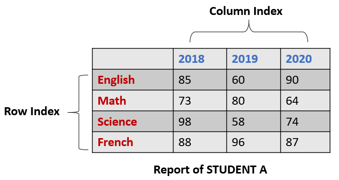
기본형태
df = pd.DataFrame(data, index, columns, dtype, copy)

데이터프레임 만들기

data = [['Choi', 22], #리스트 형태일때
        ['Kim', 48], 
        ['Joo', 32]]
df = pd.DataFrame(data, columns = ['Name', 'Age'])
print(df)

   Name  Age
0  Choi   22
1   Kim   48
2   Joo   32

data = {'Name' : ['Choi', 'Kim', 'Joo'], 'Age' : [22, 48, 32]} #딕셔너리 형태일 때
df = pd.DataFrame(data)
print(df)

   Name  Age
0  Choi   22
1   Kim   48
2   Joo   32

data = [{'a':1, 'b':2},{'a':5, 'b':10, 'c':20}]
df = pd.DataFrame(data, index = ['first', 'second'], columns = ['a', 'b'])
print(df)

        a   b
first   1   2
second  5  10

data = np.array([[1,2,3], #넘파이 데이터일때
                 [4,5,6]])
df = pd.DataFrame(data, columns = ['col1', 'col2', 'col3'])
print(df)

   col1  col2  col3
0     1     2     3
1     4     5     6

우리에게 주어진 데이터로 데이터프레임 만들기

data = {'height' : height, 'weight' : weight}
df = pd.DataFrame(data = data)
df

	height	weight
0	181	78
1	161	49
2	170	52
3	160	53
4	158	50
5	168	57
6	162	53
7	179	54
8	183	71
9	178	73
10	171	55
11	177	73
12	163	51
13	158	53
14	160	65
15	160	48
16	158	59
17	173	64
18	160	48
19	163	53
20	167	78
21	165	45
22	163	56
23	173	70
24	178	68
25	170	59
26	167	55
27	177	64
28	175	59
29	169	55
30	152	38
31	158	45
32	160	50
33	160	46
34	159	50
35	180	63
36	169	71
37	162	52
38	178	74
39	173	52
40	173	61
41	171	65
42	171	68
43	170	57
44	160	47
45	167	48
46	168	58
47	166	59
48	164	55
49	173	74
50	180	74

  <script>
    const buttonEl =
      document.querySelector('#df-734dbaa3-281d-4a1c-945f-5bb9dd901900 button.colab-df-convert');
    buttonEl.style.display =
      google.colab.kernel.accessAllowed ? 'block' : 'none';

    async function convertToInteractive(key) {
      const element = document.querySelector('#df-734dbaa3-281d-4a1c-945f-5bb9dd901900');
      const dataTable =
        await google.colab.kernel.invokeFunction('convertToInteractive',
                                                 [key], {});
      if (!dataTable) return;

      const docLinkHtml = 'Like what you see? Visit the ' +
        '<a target="_blank" href=https://colab.research.google.com/notebooks/data_table.ipynb>data table notebook</a>'
        + ' to learn more about interactive tables.';
      element.innerHTML = '';
      dataTable['output_type'] = 'display_data';
      await google.colab.output.renderOutput(dataTable, element);
      const docLink = document.createElement('div');
      docLink.innerHTML = docLinkHtml;
      element.appendChild(docLink);
    }
  </script>
</div>

회귀모델 학습시키기

OLS (Ordinary Least Square) 모듈활용
최소제곱추정법

data = {'height' : height, 'weight' : weight} #딕셔너리 형태로 만들기
df = pd.DataFrame(data = data) #데이터프레임화
df_test = pd.DataFrame(data = test_height, columns = ['height'])
model_trained = smf.ols('weight ~ height', data = df).fit() #학습할 수 있도록 모델 만들기
# model_trained = model.fit() #최소제곱추정법 적용

결과요약

y절편(b0), 기울기(b1) = intercept_coef, height_coef
결정계수 = R_squared
std err = 추정된 표준오차 $S.E(\hat\beta_{1} = \frac{s}{\sqrt{S_{xx}}})$
t = 검정통계량
P|t| = P-value

print(model_trained.summary()) #결과요약

                            OLS Regression Results                            
==============================================================================
Dep. Variable:                 weight   R-squared:                       0.542
Model:                            OLS   Adj. R-squared:                  0.533
Method:                 Least Squares   F-statistic:                     58.01
Date:                Mon, 08 May 2023   Prob (F-statistic):           7.40e-10
Time:                        00:35:31   Log-Likelihood:                -168.30
No. Observations:                  51   AIC:                             340.6
Df Residuals:                      49   BIC:                             344.5
Df Model:                           1                                         
Covariance Type:            nonrobust                                         
==============================================================================
                 coef    std err          t      P>|t|      [0.025      0.975]
------------------------------------------------------------------------------
Intercept   -100.7820     20.912     -4.819      0.000    -142.806     -58.758
height         0.9479      0.124      7.616      0.000       0.698       1.198
==============================================================================
Omnibus:                        5.480   Durbin-Watson:                   2.220
Prob(Omnibus):                  0.065   Jarque-Bera (JB):                4.425
Skew:                           0.569   Prob(JB):                        0.109
Kurtosis:                       3.886   Cond. No.                     3.75e+03
==============================================================================

Notes:
[1] Standard Errors assume that the covariance matrix of the errors is correctly specified.
[2] The condition number is large, 3.75e+03. This might indicate that there are
strong multicollinearity or other numerical problems.

$y = -100.7820 + 0.9479 \times x$

잔차제곱합 SSE 구하기

#model의 잔차를 가지고 직접 계산하기

residuals = model_trained.resid
sse = np.sum(residuals**2)

#모델에서 나오는 MSE 값으로 역으로 계산하기

mse_sse = model_trained.mse_resid * 49

print("SSE:", sse)
print("MSE SSE:", mse_sse)

SSE: 2194.852509254613
MSE SSE: 2194.852509254613

주어진 테스트 데이터로 종속변수 예측하기

df_test

predicted = model_trained.predict(df_test)
predicted

0    41.875371
1    46.614818
2    51.354265
3    56.093712
4    60.833159
5    65.572606
6    70.312053
7    75.051500
8    79.317003
dtype: float64

신뢰구간

$\hat\beta_{1}\pm t_{a/2}(n-2)\times \frac{s}{\sqrt{S_{xx}}}$

print(model_trained.conf_int(0.05)) #95% 신뢰수준에서의 신뢰구간

                    0          1
Intercept -142.806014 -58.757955
height       0.697793   1.197985

데이터 시각화하기

plt.figure(figsize=(15, 4))

plt.subplot(1, 3, 1)
slope, intercept = np.polyfit(height, weight, 1)
abline_values = [slope * i + intercept for i in height]
plt.plot(height, weight, 'o', alpha = 0.5, label = 'true data') #동그랗게 그려줘~
plt.plot(test_height, predicted, 'o', label = 'predicted data')
plt.plot(height, abline_values, 'b', label = 'line predicted')
plt.title('line suitablility')
plt.legend()
plt.xlabel('height')
plt.ylabel('weight')
plt.tight_layout()

plt.subplot(1, 3, 2)
r = model_trained.resid
plt.plot(height, r, 'o', alpha = 0.5, label = 'residuals')
plt.title('residuals')
plt.legend()
plt.xlabel('height')
plt.ylabel('weight')
plt.tight_layout()

plt.subplot(1, 3, 3)
stats.probplot(r, dist = 'norm', plot = pylab)
plt.title('Normal Probability Plot of Residual')
plt.xlabel('Theoretical Quantiles')
plt.ylabel('Sample Quantiles')
plt.tight_layout()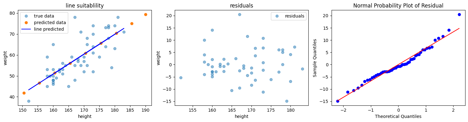

Jihwan Oh

Deep Learning, Multi-Agent RL, Large Language Model, Statistics

이전 포스트

이항분포의 정규분포화

다음 포스트

Regression (회귀분석)

data analysis

모듈 불러오기

데이터 만들기

DataFrame 패키지

데이터프레임 만들기

우리에게 주어진 데이터로 데이터프레임 만들기

회귀모델 학습시키기

결과요약

$y = -100.7820 + 0.9479 \times x$

잔차제곱합 SSE 구하기

주어진 테스트 데이터로 종속변수 예측하기

신뢰구간

데이터 시각화하기

이항분포의 정규분포화

Logistic Regression

0개의 댓글

관련 채용 정보

	height	weight
0	181	78
1	161	49
2	170	52
3	160	53
4	158	50
5	168	57
6	162	53
7	179	54
8	183	71
9	178	73
10	171	55
11	177	73
12	163	51
13	158	53
14	160	65
15	160	48
16	158	59
17	173	64
18	160	48
19	163	53
20	167	78
21	165	45
22	163	56
23	173	70
24	178	68
25	170	59
26	167	55
27	177	64
28	175	59
29	169	55
30	152	38
31	158	45
32	160	50
33	160	46
34	159	50
35	180	63
36	169	71
37	162	52
38	178	74
39	173	52
40	173	61
41	171	65
42	171	68
43	170	57
44	160	47
45	167	48
46	168	58
47	166	59
48	164	55
49	173	74
50	180	74

	height	weight
0	181	78
1	161	49
2	170	52
3	160	53
4	158	50
5	168	57
6	162	53
7	179	54
8	183	71
9	178	73
10	171	55
11	177	73
12	163	51
13	158	53
14	160	65
15	160	48
16	158	59
17	173	64
18	160	48
19	163	53
20	167	78
21	165	45
22	163	56
23	173	70
24	178	68
25	170	59
26	167	55
27	177	64
28	175	59
29	169	55
30	152	38
31	158	45
32	160	50
33	160	46
34	159	50
35	180	63
36	169	71
37	162	52
38	178	74
39	173	52
40	173	61
41	171	65
42	171	68
43	170	57
44	160	47
45	167	48
46	168	58
47	166	59
48	164	55
49	173	74
50	180	74

Regression (회귀분석)

data analysis

모듈 불러오기

데이터 만들기

DataFrame 패키지

데이터프레임 만들기

우리에게 주어진 데이터로 데이터프레임 만들기

회귀모델 학습시키기

결과요약

y=−100.7820+0.9479×xy = -100.7820 + 0.9479 \times xy=−100.7820+0.9479×x

잔차제곱합 SSE 구하기

주어진 테스트 데이터로 종속변수 예측하기

신뢰구간

데이터 시각화하기

이항분포의 정규분포화

Logistic Regression

0개의 댓글

관련 채용 정보

$y = -100.7820 + 0.9479 \times x$

	height	weight
0	181	78
1	161	49
2	170	52
3	160	53
4	158	50
5	168	57
6	162	53
7	179	54
8	183	71
9	178	73
10	171	55
11	177	73
12	163	51
13	158	53
14	160	65
15	160	48
16	158	59
17	173	64
18	160	48
19	163	53
20	167	78
21	165	45
22	163	56
23	173	70
24	178	68
25	170	59
26	167	55
27	177	64
28	175	59
29	169	55
30	152	38
31	158	45
32	160	50
33	160	46
34	159	50
35	180	63
36	169	71
37	162	52
38	178	74
39	173	52
40	173	61
41	171	65
42	171	68
43	170	57
44	160	47
45	167	48
46	168	58
47	166	59
48	164	55
49	173	74
50	180	74