[논문정리] Video Textures

Abstract

이 논문은 새로운 medium 인 video texture 에 대해 소개하고, video clip 을 분석해 구조를 추출하고 임의 길이의 비슷하게 보이는 새로운 비디오를 합성하는 기술을 제시한다.

video texture 와 view morphing 기술을 결합하여 3D video textures 를 얻을 수 있고, video textures 합성이 높은 수준의 대화형 controls를 통해 사용자가 가이드할 수 있는 video-based animation에 대해 소개한다. 더 나아가 video textures 의 applications 와 extensions도 다룬다.

1. Introduction

picture is worth a thousand words! 😀 하지만 정적인 사진으로 표현할 수 없는 것들이 있다. (떨어지는 폭포나 바람에 펄럭이는 깃발과 같이,,)
→ 이런 정적인 사진을 대체할 만한 것은 video ✨.

💢 하지만 video 도 단점이 있는데 video를 저장하고 싶으면 finite duration 인 video clip 으로 만들어서 저장을 해야한다. 즉, 시간에 따라 변화하는 현상을 표현할 수 있지만, 사진의 "timeless"한 quality가 부족하다.

💡 그래서 이 논문에서는 사진과 비디오의 중간이라고 할 수 있는 새로운 medium 타입을 제시한다. ⇒ Video Texture✨

video texture 는 continuous, infinitely varying stream of video images를 제공한다. 그리고 source video에서 원본 프레임을 무작위로 rearranging(및 blending)하여 finite한 image set 에서 합성된다.

• Video texture’s applicability.

  • 기존 비디오 플레이어 및 웹 브라우저와의 하위 호환성을 위해, 눈에 보이는 불연속성 없이 계속 재생하도록 유한한 지속 시간 video loops 를 생성할 수 있다.
  • 원본 비디오는 독립적으로 움직이는 regions 로 분할될 수 있으며, 각 region 은 독립적으로 analyzed 및 rendered 될 수 있다.
  • 또한 컴퓨터 비전 기술을 사용하여 배경에서 objects 를 분리하고 임의의 이미지 위치에서 렌더링할 수 있는 video sprites 로 나타낼 수 있다.
  • stereo matching 및 view morphing 기술과 결합하여 3-dim video textures를 생성할 수도 있다.
  • video-based animation.

• Problems

  • video sequences 에서 잠재적인 transition points를 찾는 것. (i.e. places where the video can be looped back on itself in a minimally obtrusive way.)
  • 비디오 전체 구조를 respects 하는 transitions sequence를 찾는 것.
  • transitions시 시각적 불연속성을 부드럽게 하는 것(By using morphing techniques.)
  • 비디오 프레임을 독립적으로 분석 및 합성할 수 있는 다른 영역으로 자동 factoring 하는 것.
  • +$\alpha$

1.1 Related work

• Video-based rendering
• Video Rewrite
• Video sprite
• Video clip-art
• temporal extension of 2D image texture synthesis.

1.2 System overview

👀 Q. Given a small amount of “training video” (our input video clip), how do we generate an infinite amount of similar looking video?
😀 A. find places in the original video where a transition can be made to some other place in the video clip without introducing noticeable discontinuities.

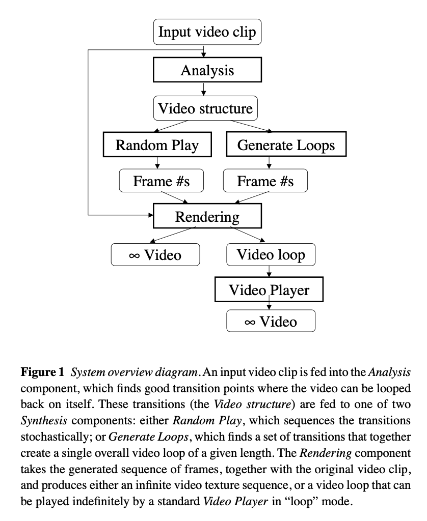
• Three major components

  1. The first component of the system analyzes the input video to find the good transition points, and stores these in a small data table that becomes part of the video texture representation.

  2. The second component of our system synthesizes new video from the analyzed video clip, by deciding in what order to play the original video frames.

     (Random Play or Generate Loops)

  3. The last component of our system is rendering component that puts together the frames in a way that is visually pleasing.

Section 2) More detail about the representation used to capture the structure of video textures.

Section 3) Our process for extracting this representation from source video.

Section 4) Synthesizing the video texture.

Section 5) Rendering algorithms.

Section 6) The discussion of our basic results

Section 7) Description of some further extensions

2. Representation

• Our video textures are essentially Markov processes

  • each state corresponding to a single video frame
  • the probabilities corresponding to the likelihood of transitions from one frame to another.

• Video Textures 저장이 유용한 representation.

  1. matrix of probabilities (Figure 3)
     • each element $P_{ij}$ : frame $i$ 에서 frame $j$ 로 transitioning 하는 것의 확률.
  2. set of explicit links(Figure 6) from one frame $i$ to another $j$, along with an associated probability.

3. Analysis: Extracting the video texture

😀 The first step in creating a video texture from an input video sequence is to compute some measure of similarity between all pairs of frames in the input sequence. → using $L_2$ distance✨

frame-to-frame distances 계산 후 matrix에 저장.

로운 비디오 합성할 때 기본 아이디어는 $i$의 successor 가 $j$와 유사할 때마다, 즉 $D_{i+1,j}$가 작을 때마다 frame $i$에서 frame $j$로의 transitions를 생성하는 것이다.

이를 수행하는 간단한 방법은 지수 함수를 통해 이러한 거리를 확률에 매핑하는 것이다.

$P$의 주어진 행에 대한 모든 확률은 $\sum_{j}P_{ij} = 1$ 이 되도록 normalized 되고, $P_{ij}$의 분포에 따라 frame $i$ 다음에 표시할 next frame이 선택된다.

• $σ$ parameter controls the mapping between $L_2$ distance and relative probability of taking a given transition.
  • $σ$ 의 값이 작을수록 가장 좋은 transition 만 강조.
  • $σ$ 의 값이 클수록 transition 이 좋지 않은 대신 더 큰 다양성을 허용.

→ We typically set $σ$ to a small multiple of the average $D_{ij}$ values, so that the likelihood of making a transition at a given frame is fairly low.

3.1 Preserving dynamics

😀 video textures는 frames간의 similarity 뿐만 아니라 dynamics of motion 도 보존해야 한다.

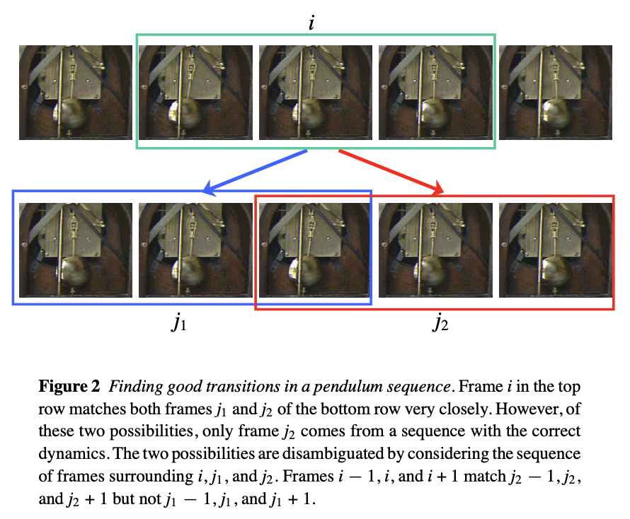
예를 들어 Figure2 의 흔들리는 진자(swinging pendulum)를 봐보자.

left-to-right swing 의 각 frame은 그와 대응해서 매우 유사하게 보이는 right-to-left swing 프레임이 있다. (파란색 화살표로 표시)

그러나, left-to-right swing의 frame $i$ 에서 $i+1$과 매우 유사한 right-to-left swing의 frame 으로 transitioning 하는 것은 진자의 움직임에 abrupt and unacceptable한 변화를 발생시킨다.

We solve the problem of preserving dynamics by also requiring temporally adjacent frames within some weighted window must be similar to each other.

즉, individual frames 대신 subsequences를 일치시킨다. 이러한 subsequences 일치는 weights $[w_{-m},...,w_{m-1} ]$ 가 있는 diagonal kernel 로 difference matrix를 필터링하여 달성할 수 있다.

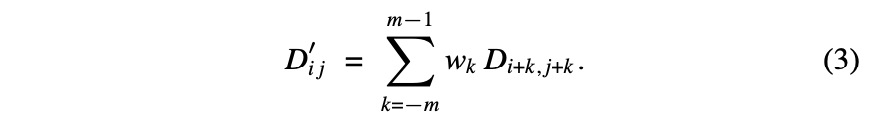
실제 적용할때, 우리는 binomial weights 와 함께 2- or 4- tap filter에 해당하는 $m =$ 1 or 2를 사용한다.

(필터를 짝수 길이로 만들면 asymmetry 를 제거하면서, $i + 1$ 과 $j$의 similarity 만큼 $i$ 와 $j−1$의 similarity 에 의해 결정되는 일부 프레임 $i$에서 일부 다른 프레임 $j$로의 transition 결정이 허용된다. )

filtered difference matrix 에서 확률을 필터링하고 계산한 후에는, the undesired transitions no longer have high probability.

👀 Figure 3은 Figure 2의 pendulum sequence에 대해 $D_{ij}$ 와 $P_{ij}$ 테이블의 2차원 이미지를 사용하여 이 동작을 보여준다.

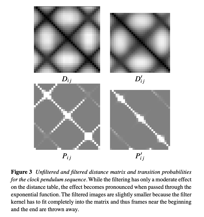
• The original unfiltered tables: 진자의 주기적인 특성을 쉽게 볼 수 있으며 forward 와 backward swings 을 모두 일치시키는 경향이 있다.
• After filtering : 같은 방향의 swings 만 매칭한다. (밝은 knots는 진자가 스윙의 끝에서 멈추는 것을 나타내고, 더 많은 self-similarity 를 갖는 곳이다.)

3.2 Avoiding dead ends and anticipating the future

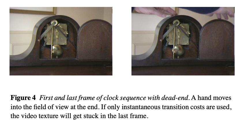
😀 The decision rule we have described so far tries to match the appearance and dynamics in the two frames, but gives no consideration to whether the transition might lead to some portion of the video from which there is no graceful exit—a “dead end,” in effect (Figure 4).

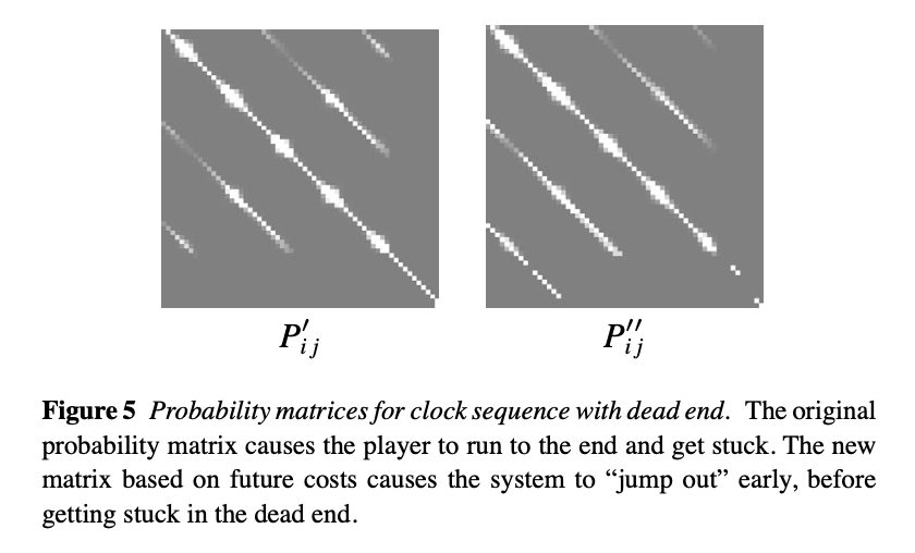
💡 Planning ahead : future transitions를 고려해서, 주어진 transitions를 선택하는 데 예상되는(증가한) "future cost"를 예측.

• $D''_{ij}$ : anticipated future cost of a transition from frame $i-1$ to frame $j$. (i.e. cost that reflects the expected average cost of future transitions)

• $p$ : 여러 좋은(low-cost) transition 과 하나의 poorer transition 사이의 tradeoff 를 제어하는 데 사용되는 constant. ($p$가 높을수록 여러 좋은 전환을 선호, $p$가 낮을수록 하나의 불량한 전환을 선호.)
• $\alpha$ : metric에서 future transitions 의 상대적 가중치를 제어하는 데 사용되는 constant. (for convergence, we must choose 0 < $α$ < 1 (in practice, we use 0.99 ≤ $α$ ≤ 0.999).)

😢 식 (4), (5)번을 교대로 일어나게 하는 알고리즘은 수렴하기가 굉장히 느리다.

$σ → 0$ 이면, 식 (5)번의 $P''_{jk}$ 은 best transition은 1, 나머지는 0 으로 될 수 있기 때문에 식 (4)번을 아래와 같이 대신할 수 있다.

3.3 Pruning the transitions

😀 It is often desirable to prune the set of allowable transitions, both to save on storage space, and to improve the quality of the resulting video (suppressing non-optimal transitions).

• Two pruning paradigms:
  1. Select only local maxima in the transition matrix for a given source and/or destination frame.
     • transition matrix 에서 frame의 주변 frame들이 모두 비슷하게 좋은 transition을 가지고 있으면 하나만 골라서 "sweet spots” 으로 정한다.
  2. Set all probabilities below some threshold to zero.

4. Synthesis: Sequencing the video texture

😀 Once the analysis stage has identified good transitions for the video texture, we need to decide in what order to play the video frames.

• Synthesis stage:
  • Random Play algorithms
  • Video Loops algorithms

Random Play

The video texture is begun at any point before the last non-zero-probability transition.

After displaying frame $i$ , the next frame $j$ is selected according to $P_{ij}$ . Note that usually, $P_{i,i+1}$ is the largest probability, since $D'_{ii} = 0$.

→ 이렇게 간단한 Monte-Carlo 접근 방식은 반복되지 않는 video texture 를 생성하고, source material 에서 video texture 를 즉시 생성할 수 있는 상황에서 유용하다.

4.1 Video loops

Consider a loop with a single transition $i→j$ , from source frame $i$ to destination frame $j$, which we call a primitive loop.

single transition이 (non-trivial)cycle를 만들려면 $i ≥ j$ 이어야 한다.

• the range of this loop is $[j, i]$.
• the cost of this loop is the filtered distance between the two frames $D'_{ij}$ **.

하나 이상의 primitive loop을 결합하여 compound loops 라고 하는 추가적인 cyclic sequences를 생성할 수 있고, loop을 추가하기 위해서는 overlap되는 range가 존재해야 한다.

💡 Our algorithm for creating compound loops of minimal average cost considers only backward transitions (transitions $i → j$ **with $i ≥ j$)

• Two algorithms to generate optimal loops:
  1. selects a set of transitions that will be used to construct the video loop.
  2. orders these transitions in a legal fashion.

4.2 Selecting the set of transitions

The most straightforward way is to enumerate all multisets of transitions of total length $L$, and to keep the best one. → exponential in the number of transitions considered. 😵

✨ Using Dynamic programming algorithm

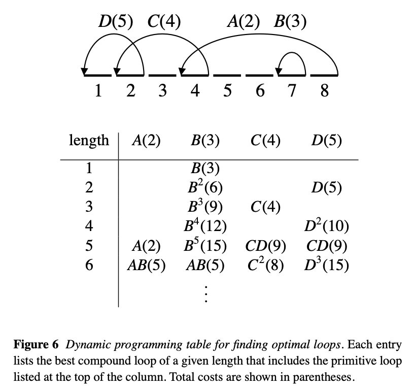
$L$ 개의 행과 $N$개의 열로 구성된 테이블을 만든다.(Figure 6) 테이블의 각 셀에는 compound loop의 transitions과 compound loop’s total cost가 나열된다.

• $L$ : maximum loop length being considered.
• $N$: the number of transitions(or primitive loop) being considered.

The algorithm builds a list of the best compound loop of a given length that contains at least one instance of the primitive loop listed at the top of the column.

The algorithm works by updating cells one row at a time.

For each cell, it examines all compound loops of shorter length in that same column, and tries to combine them with compound loops from columns whose primitive loops have ranges that overlap that of the column being considered.

For each cell, it examines all compound loops of shorter length in that same column, and tries to combine them with compound loops from columns whose primitive loops have ranges that overlap that of the column being considered.

For each of the $LN$ **cells examined, the algorithm must combine at most $L − 1$ compound loops from its column with at most $N − 1$ entries from the other columns.

→ 계산 복잡도는 $O(L^2N^2)$, 공간복잡도는 $O(LN)$ 이다.

4.3 Scheduling the primitive loops

😀 Now, the transitions have to be scheduled in some order so that they form a valid compound loop. (we use the scheduling of {$ABCD$}) :

1. sequence 의 맨 끝에서 시작하는 transition 을 첫 번째로 수행할 transition 으로 잡는다. ($A$)

2. transition $i → j$ 를 제거하는 것은 나머지 primitive loops를 하나 이상의 continuous ranges sets로 나눌 수 있다. 우리의 예시에서 $A$ 를 제거하면 나머지 loops 가 두 개의 continuous-range sets {${C, D}$}와 {${B}$}로 나뉜다. Frame $j$는 항상 첫 번째 집합에 포함되며 $j$ 이후에 source frame 이 발생하는 이 집합의 모든 transition 을 다음으로 예약한다. 이 예에서 $C$는 이러한 기준을 충족하는 유일한 transition이다.

3. 이전의 스텝을 반복하고, 첫번째 범위에서 primitive loops가 없어질 때까지 transitions $i → j$ **를 제거한다. 이 예제에서 $D$는 이 반복된 단계에 의해 다음으로 제거된다.

4. step 2에서 시작하는 알고리즘을 사용하여, 다음 각 disjoint ranges 에서 primitive loop 를 정한다. ****이 예제에서는 유일한 primitive loop $B$가 남는다.

5. 모든 primitive loops 가 제거될 때까지 step 2 를 계속한다.

⇒ In our example, the loops are scheduled in the order $A, C, D, B$.

The computational complexity of this algorithm is quadratic in the number of transitions in the compound loop. The scheduling algorithm can either be run in a deterministic fashion or in a stochastic fashion.

The latter variant, which utilizes transitions with precisely the same frequency as in the compound loop, is an alternative to the Monte-Carlo sequencing algorithm presented earlier.

5. Rendering

😀 This section describes techniques for disguising discontinuities in the video texture, and for blending independently analyzed regions together.

• Cross-fading
  • The images of the sequence before and after the transition can be blended together with standard cross-fading:
  • frames from the sequence near the source of the transition are linearly faded out as the frames from the sequence near the destination are faded in.
  • The fade is positioned so that it is halfway complete where the transition was scheduled.
  • Although cross-fading of the transitions avoids abrupt image changes, it temporarily blurs the image if there is a misalignment between the frames. The transition from sharp to blurry and back again is sometimes noticeable. In some situations, this problem can be addressed by taking very frequent transitions so that several frames are always being cross-faded together, maintaining a more or less constant level of blur.
  • Our implementation of the cross-fading algorithm supports multiway cross-fades, i.e., more than two subsequences can be blended together at a time. The algorithm computes a weighted average of all frames participating in a multi-way fade,

• Morphing
  • morph the two sequences together, so that common features in the two sets of frames are aligned. The method we use is based on the de-ghosting algorithm and is also related to automatic morphing techniques.
  • To perform the de-ghosting, we first compute the optical flow between each frame $I_i$participating in the multi-way morph and a reference frame $I_R$ **(the reference frame is the one that would have been displayed in the absence of morphing or cross-fading).
  • For every pixel in $I_R$ , we find a consensus position for that pixel by taking a weighted average of its corresponding positions in all of the frames $I_i$ (including $I_R$ **).
  • Finally, we use a regular inverse warping algorithm to resample the images such that all pixels end up at their consensus positions.
  • We then blend these images together.

6. Basic results

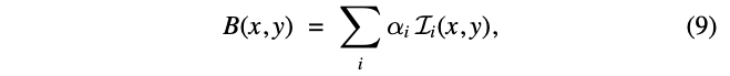
Candle flame. A 33-second video of a candle flame was turned into four different video textures: one random play texture; and three different video loops, each containing three different primitive loops. One of the video loops repeats every 426 frames. The other two repeat every 241 frames; these each use the same set of three primitive loops, but are scheduled in a different order.

In the figure, the position of the frame currently being displayed in the original video clip is denoted by the red bar. The red curves show the possible transitions from one frame in the original video clip to another, used by the random play texture.

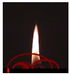
Campfire. A 10-second video of a campfire was cyclified using a single transition. The transition is hardly visible without cross-fading, but cross-fading over four frames hides it entirely. Although the configuration of the flames never replicates even approximately, the transition is well hidden by the high temporal flicker.

7. Extensions

we present several extensions to the basic idea of video textures.

7.1 Sound synthesis

😀 audio track is rerendered along with the video texture.

video textures 에 sound 를 추가하는 것은 비교적 간단한데 각 프레임과 관련된 sound samples 를 가져와서 렌더링하도록 선택한 video frame 과 함께 재생하기만 하면 된다.

7.2 Three-dimensional video textures

😀 view interpolation techniques are applied to simulate 3D motion.

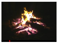
3D Portrait. We created a three-dimensional video texture from three videos of a smiling woman, taken simultaneously from three different viewing angles about 20 degrees apart. We used the center camera to extract and synthesize the video texture, and the first still from each camera to estimate a 3D depth map, shown here.

We then masked out the background using background subtraction (a clear shot of the background was taken before filming began). To generate each new frame in the 3D video animation, we mapped a portion of the video texture onto the 3D surface, rendered it from a novel view-point, and then combined it with the flat image of the background warped to the correct location.

7.3 Motion factorization

😀 the video frames are factored into separate parts that are analyzed and synthesized independently. This kind of motion factorization decreases the number of frame samples necessary to synthesize an interesting video texture.

The simplest form of motion factorization is to divide the frame into independent regions of motion, either manually or automatically.

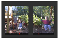
Swings. In this example, the video of two children on swings is manually divided into two halves: one for each swing. These parts are analyzed and synthesized independently, then recombined into the final video texture. The overall video texture is significantly superior to the best video texture that could be generated using the entire video frame.

Motion factorization can be further extended to extract independent video sprites from a video sequence.

Fish. We used background subtraction to create a video sprite of a fish, starting from 5 minutes of video of a fish in a tank. Unfortunately, fish are uncooperative test subjects who frequently visit the walls of the fish tank, where they are hard to extract from the scene because of reflections in the glass. We therefore used as source material only those pieces of video where the fish is swimming freely. (This requires generalizing the future cost computation to handle the possibility of multiple dead ends, but is otherwise straightforward.)

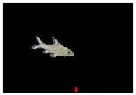
Using this technique, the fish swims freely in two-dimensional space. Ideally, we would like to constrain its motion—for example, to the boundaries of a fish tank.

7.4 Video-based animation

😀 Instead of using visual smoothness as the only criterion for generating video, we can also add some user-controlled terms to the error function in order to influence the selection of frames.

The simplest form of such user control is to interactively select the set of frames S in the sequence that are used for synthesis.

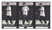
Runner. We took 3 minutes of video of a runner on a treadmill, starting at a slow jog and then gradually speeding up to a fast run. As the user moves a slider selecting a certain region of the video (the black region of the slider in the figure), the synthesis attempts to select frames that remain within that region, while at the same time using only fairly smooth transitions to jump forward or backward in time. The user can therefore control the speed of the runner by moving the slider back and forth, and the runner makes natural-looking transitions between the different
gaits.

8. Discussion and future work

• Better distance metrics.
• Better Blending.
• Maintaining variety
• Better tools for creative control.

https://dl.acm.org/doi/abs/10.1145/344779.345012