https://arxiv.org/abs/1506.02640

Abstract

YOLO, a new approach to object detection.✨
we frame object detection as a regression problem to spatially separated bounding boxes and associated class probabilities.

Since the whole detection pipeline is a single network, it can be optimized end-to-end directly on detection performance.

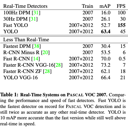
• YOLO model processes images in real-time at 45 frames per second. A smaller version of the network, Fast YOLO, processes an astounding 155 frames per second while still achieving double the mAP of other real-time detec- tors.
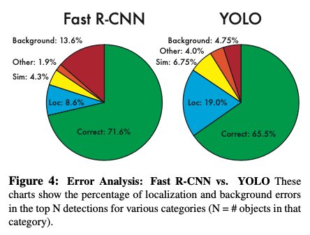
• Compared to state-of-the-art detection systems, YOLO makes more localization errors but is less likely to predict false positives on background.
• Finally, YOLO learns very general representations of objects.

1. Introduction

Current detection systems repurpose classifiers to perform detection. To detect an object, these systems take a classifier for that object and evaluate it at various locations and scales in a test image.

• Systems like deformable parts models (DPM) use a sliding window approach where the classifier is run at evenly spaced locations over the entire image.
• More recent approaches like R-CNN use region proposal methods to first generate potential bounding boxes in an image and then run a classifier on these proposed boxes. After classification, post-processing is used to refine the bounding boxes, eliminate duplicate detections, and rescore the boxes based on other objects in the scene. These complex pipelines are slow and hard to optimize because each individual component must be trained separately.

✨ We reframe object detection as a single regression problem, straight from image pixels to bounding box coordinates and class probabilities.
Using our system, you only look once (YOLO) at an image to predict what objects are present and where they are.

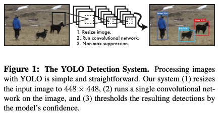
😀 YOLO is refreshingly simple (Figure 1)
A single convolutional network simultaneously predicts multiple bounding boxes and class probabilities for those boxes. YOLO trains on full images and directly optimizes detection performance.

This unified model has several benefits over traditional methods of object detection.

• First, YOLO is extremely fast. Since we frame detection as a regression problem, we simply run our neural network on a new image at test time to predict detections. Furthermore, YOLO achieves more than twice the mean average precision of other real-time systems.
• Second, YOLO reasons globally about the image when making predictions. YOLO sees the entire image during training/test time so it implicitly encodes contextual information about classes as well as their appearance.
• Third, YOLO learns generalizable representations of objects. It is less likely to break down when applied to new domains or unexpected inputs.

😢 YOLO still lags behind state-of-the-art detection systems in accuracy. While it can quickly identify objects in images it struggles to precisely localize some objects, especially small ones.

2. Unified Detection

We unify the separate components of object detection into a single neural network.

• Uses features from the entire image to predict each bounding box.
• It also predicts all bounding boxes across all classes for an image simultaneously.
• YOLO design enables end-to-end training and real-time speeds while maintaining high average precision.

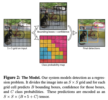
Our system divides the input image into an S × S grid.
Each grid cell predicts B bounding boxes and confidence scores for those boxes.

• These confidence scores reflect how confident the model is that the box contains an object and also how accurate it thinks the box is that it predicts.
• we define confidence as $Pr(Object) ∗ IOU^{truth}_{pred}$.
• If no pred object exists in that cell, the confidence scores should be zero.
• Otherwise we want the confidence score to equal the intersection over union (IOU) between the predicted box and the ground truth.

• Each bounding box consists of 5 predictions: x, y, w, h, and confidence.

  • The (x, y) coordinates represent the center of the box relative to the bounds of the grid cell.
  • The width and height are predicted relative to the whole image.
  • Finally the confidence prediction represents the IOU between the predicted box and any ground truth box.

• Each grid cell also predicts C conditional class probabilities, $Pr(Class_i |Object)$. These probabilities are conditioned on the grid cell containing an object. We only predict one set of class probabilities per grid cell, regardless of the number of boxes B.

• At test time we multiply the conditional class probabilities and the individual box confidence predictions, which gives us class-specific confidence scores for each box.
  These scores encode both the probability of that class appearing in the box and how well the predicted box fits the object.
  

For evaluating YOLO on PASCAL VOC, we use S = 7, B = 2. PASCAL VOC has 20 labelled classes so C = 20. Our final prediction is a 7 × 7 × 30 tensor.

2.1. Network Design

We implement this model as a convolutional neural network and evaluate it on the PASCAL VOC detection dataset.

• The initial convolutional layers of the network extract features from the image.
• The fully connected layers predict the output probabilities and coordinates.

Our network architecture is inspired by the GoogLeNet.
(The full network is shown in Figure 3.)

• 24 convolutional layers followed by 2 fully connected layers.
• Instead of the inception modules, we simply use 1 × 1 reduction layers followed by 3 × 3 convolutional layers.

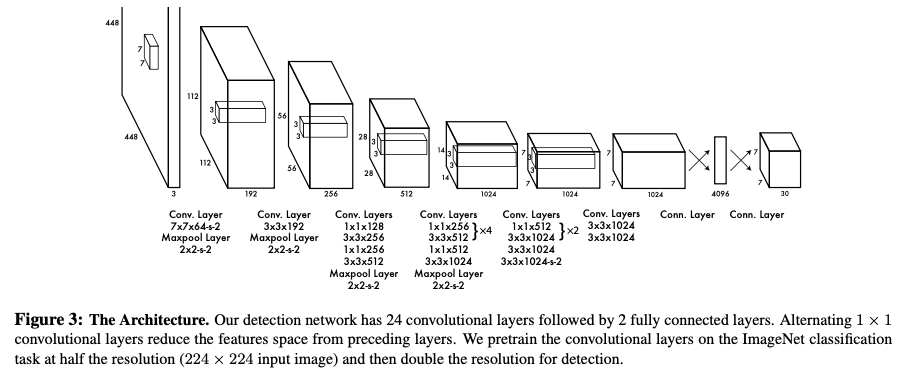
The final output of our network is the 7 × 7 × 30 tensor of predictions.

2.2. Training

1. We pretrain our convolutional layers on the ImageNet 1000-class competition dataset. For pretraining we use the first 20 convolutional layers from Figure 3 followed by a average-pooling layer and a fully connected layer.
   We achieve a single crop top-5 accuracy of 88% on the ImageNet 2012 validation set, comparable to the GoogLeNet models in Caffe’s Model Zoo.
   We use the Darknet framework for all training and inference.

2. We then convert the model to perform detection. We add four convolutional layers and two fully connected layers with randomly initialized weights.
   Detection often requires fine-grained visual information so we increase the input resolution of the network from 224 × 224 to 448 × 448.

3. Our final layer predicts both class probabilities and bounding box coordinates.
   We normalize the bounding box width and height by the image width and height so that they fall between 0 and 1. We parametrize the bounding box x and y coordinates to be offsets of a particular grid cell location so they are also bounded between 0 and 1.

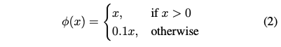
We use a linear activation function for the final layer and all other layers use the following leaky rectified linear activation:

We optimize for sum-squared error in the output of our model, because it is easy to optimize
💢However it does not perfectly align with our goal of maximizing average precision.

• It weights localization error equally with classification error which may not be ideal.
• Also, in every image many grid cells do not contain any object. This pushes the “confidence” scores of those cells towards zero, often overpowering the gradient from cells that do contain objects. This can lead to model instability, causing training to diverge early on.

😀 To remedy this, we increase the loss from bounding box coordinate predictions and decrease the loss from confi- dence predictions for boxes that don’t contain objects.
→ Using two parameters, $λ_{coord} = 5$ and $λ_{noobj} = 5$.

💢 Sum-squared error also equally weights errors in large boxes and small boxes. Our error metric should reflect that small deviations in large boxes matter less than in small boxes.
😀 To partially address this we predict the square root of the bounding box width and height instead of the width and height directly.

💢 YOLO는 grid cell 당 multiple bounding boxes를 예측하는데, training 때 우리는 객체에 responsible한 one bounding box predictor만 필요하다. (We assign one predictor to be “responsible” for predicting an object based on which prediction has the highest current IOU with the ground truth.)
😀 This leads to specialization between the bounding box predictors. Each predictor gets better at predicting certain sizes, aspect ratios, or classes of object, improving overall recall.

During training we optimize the following, multi-part loss function:

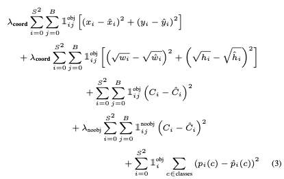
where $\mathbb{1^{obj}_i}$ denotes if object appears in cell $i$ and $\mathbb{1^{obj}_{ij}}$ denotes that the $j$th bounding box predictor in cell $i$ is “responsible” for that prediction.

The loss function only penalizes classification error if an object is present in that grid cell.
It also only penalizes bounding box coordinate error if that predictor is “responsible” for the ground truth box (i.e. has the highest IOU of any predictor in that grid cell).

• We train the network for about 135 epochs on the training and validation data sets from PASCAL VOC 2007 and 2012.

• When testing on 2012 we also include the VOC 2007 test data for training.

• batch size of 64 while training

• a momentum of 0.9

• a decay of 0.0005.

learning rate schedule
For the first epochs we slowly raise the learning rate from 10−3 to 10−2. We continue training with 10−2 for 75 epochs, then 10−3 for 30 epochs, and finally 10−4 for 30 epochs.

overfitting

• Dropout
• Extensive data augmentation.(random scaling and translations)

2.3. Inference

✨ Just like in training, predicting detections for a test image only requires one network evaluation.

Often it is clear which grid cell an object falls in to and the network only predicts one box for each object.
However, some large objects or objects near the border of multiple cells can be well localized by multiple cells.
Non-maximal suppression can be used to fix these multiple detections.

2.4. Limitations of YOLO

• spatial constraints on bounding box predictions.
• Struggles to generalize to objects in new or unusual aspect ratios or configurations.
• Loss function treats errors the same in small bounding boxes versus large bounding boxes.

3. Comparison to Other Detection Systems

1. Deformable parts models.

• Deformable parts models (DPM) use a sliding window approach to object detection.
• DPM uses a disjoint pipeline to extract static features, classify regions, predict bounding boxes for high scoring regions, etc.

→ YOLO is a single convolutional neural network.✨
→ faster, more accurate ✨
Instead of static features, the network trains the features in-line and optimizes them for the detection task.

2. R-CNN.
R-CNN and its variants use region proposals to find objects in images.
This complex pipeline must be precisely tuned independently and the resulting system is very slow.😵

→ YOLO puts spatial constraints on the grid cell proposals which helps mitigate multiple detections of the same object.✨
→ YOLO proposes far fewer bounding boxes, only 98 per image compared to about 2000 from Selective Search. ✨
→ YOLO combines these individual components into a single, jointly optimized model.

3. Other Fast Detectors

4. Experiments

4.1. Comparison to Other Real-Time Systems

4.2. VOC 2007 Error Analysis

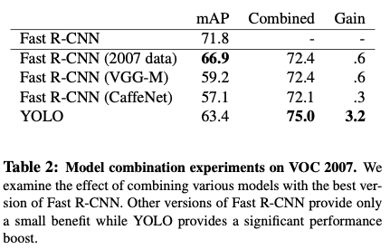
4.3. Combining Fast R-CNN and YOLO

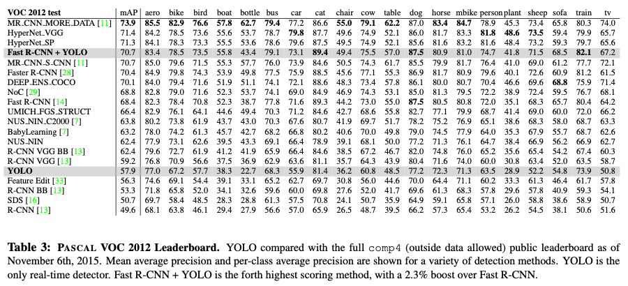
4.4. VOC 2012 Results

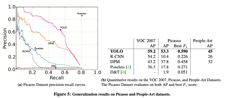
4.5. Generalizability: Person Detection in Artwork

5. Real-Time Detection In The Wild

6. Conclusion

We introduce YOLO, a unified model for object detection.
🌸 YOLO is simple to construct
🌸 YOLO can be trained directly on full images.
🌸 YOLO is trained on a loss function that directly corresponds to detection performance
🌸 Entire model is trained jointly.
🌸 Fast YOLO is the fastest general-purpose object detector in the literature.
🌸 YOLO pushes the state-of-the-art in real-time object detection.
🌸 YOLO also generalizes well to new domains making it ideal for applications that rely on fast, robust object detection.