[ML] 3. Classification (1)

앙버터·2023년 11월 5일

ML

목록 보기

1/10

1. MNIST

7만개의 작은 숫자 이미지 (손글씨)
각 이미지는 라벨링되어있음(숫자)

from sklearn.datasets import fetch_openml
mnist = fetch_openml('mnist_784', version=1, as_frame=False)
mnist.keys()
>> dict_keys(['data', 'target', 'frame', 'categories', 'feature_names', 'target_names', 'DESCR', 'details', 'url'])

DESCR : 데이터셋 설명
data : instance(행, row) / feature(열, column)
target : label 배열을 담은 key

👉 data : 7만(각 이미지) * 784(특성 개수=28x28pixel)
👉 target : 7만(label 개수, 각 이미지당 1개)

각 특성 하나는 0~255(흰~검)의 값을 지님(=pixel intensities)

이미 순서대로 정렬되어 있음 : training(앞 6만)/test(뒤 1만)

	X_train, X_test, y_train, y_test = X[:60000], X[60000:], y[:60000], y[60000:]

shuffling : for CV, 이미 완료되어 있음

2. Binary classifier 훈련

2.1 5-detector : 2 classes (5 or not 5)

y_train_5 = (y_train == 5)
y_test_5 = (y_test == 5)

SGD(확률적 경사 하강법) 이용
-매우 큰 데이터를 효율적으로 처리 가능 (한 번에 한 개의 샘플을 독립적으로 처리)
✔ 독립적으로 처리하기 때문에 셔플링된 MNIST를 사용함
-무작위성(randomness)에 의존

from sklearn.linear_model import SGDClassifier

sgd_clf = SGDClassifier(random_state=42) #항상 동일한 결과를 출력
sgd_clf.fit(X_train, y_train_5)

sgd_clf.predict([some_digit]) #some_digit = X[0]
>> array([ True])

✔ 5(True, Positive class) <-> not 5(False, Negative class)

3. Performance Measure

3.1 Accuracy

classifier에 대해 선호하지 않음
불균형 데이터셋의 경우 클래스 치우침 현상으로 정확도가 무조건 높게 나올 수 있다.

3.2 Cross-Validation

k-fold CV
1)training set을 k개로 나눈다
2)1번 fold를 evaluation에 사용, 나머지로 training
2번 fold를 evaluation에 사용, 나머지로 training
... ▶ k번 학습+평가 진행

ex. 3-fold
```
cross_val_score(sgd_clf, X_train, y_train_5, cv=3, scoring="accuracy")
>> array([0.95035, 0.96035, 0.9604 ])
```
각 fold에서 얻은 accuracy 반환 (scoring="accuracy")

Dummy classifier (Never5classifier)
모두 not 5로 예측하는 분류기 (결과 항상 False)

class Never5Classifier(BaseEstimator):
	def fit(self, X, y=None):
 		pass
    def predict(self, X):
    		return np.zeros((len(X), 1), dtype=bool)
         
from sklearn.dummy import DummyClassifier
dummy_clf = DummyClassifier()
dummy_clf.fit(X_train, y_train_5)
cross_val_score(dummy_clf, X_train, y_train_5, cv=3, scoring="accuracy")
>> array([0.90965, 0.90965, 0.90965])

MNIST는 0~9까지 10개의 숫자가 존재하므로, 5는 10%, not 5는 90% 로 나눌 수 있다.
✔ 각 class가 비슷한 비율의 dataset을 가지고 있어야 일관적인 학습에 용이하다.

random number를 도출하는 경우 정확도는 50%이므로
분류기는 50% ~ 100%의 정확도를 갖는다.

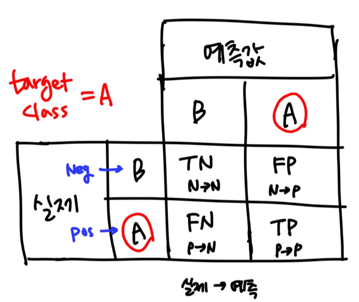
3.3 Confusion Matrix

클래스 A의 샘플이 클래스 B로 분류된 횟수를 세는 것
1) 예측값 생성
cross_val_predict : k-fold CV 진행. score대신 각 test fold에서 얻은 예측값을 반환한다.

  	from sklearn.model_selection import cross_val_predict
      y_train_pred = cross_val_predict(sgd_clf, X_train, y_train_5, cv=3)

"clean" prediction : 학습에 사용되지 않은 데이터에 대해 얻어진 예측값 (input = X_train)

2) 교차 검증(cross-validation) 진행
: confusion_matrix(target, prediction) 사용

	from sklearn.metrics import confusion_matrix
	cm = confusion_matrix(y_train_5, y_train_pred)
	>array([[53892,   687],
	       [ 1891,  3530]])

(True/False) : 맞냐/틀리냐
(Pos/Neg) : 예측 결과

첫번째 행 : non-5 (실제 값=Negative)
True Negative(TN) = N->N correct
False Positive(FP) = N->P

두번째 행 : 5 (실제 값=Positive)
False Negative(FN) = P->N
True Positive(TP) = P->P correct

perfect classifier : P->P / N->N (correct)
precision = recall = 1 이며, 존재하지 않는다.

# 대각행렬(diagonal matrix)로 나타남
array([[54579,     0],
       [    0,  5421]])

정밀도(precision) & 재현율(recall)
✅ Precision : positive로 예측된 것들 중 -> positive로 예측된 비율
precision_score = TP/(TP+FP)
✅ Recall : 실제값이 positive인 것들 중 -> positive로 예측된 비율
recall_score = TP/(TP+FN)
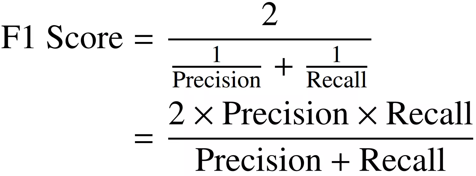
✅ F1 score : precision과 recall의 조화평균
f1_score
precision과 recall이 비슷한 경우 -> 높은 F1 score
상황에 따라 precision이 중요할 수도 있고, recall이 중요할 수도 있다.
- detect kid-safe video
  높은 precision : 안전한 영상만 보이도록 한다.
  낮은 recall : 좋은 영상이 거부될 수 있다.
- detect shoplifters on surveillance images
  높은 recall : 강도로 인식되는 실제 강도가 많아짐
  낮은 precision : 강도가 아닌데 인식되는 경우가 많아짐 (가짜 경고가 늘어남)
  ✔ recall 100% - 모든 실제 강도가 강도로 인식됨
  ➡ 이는 '은행을 들어갈 때 불편함이 생기더라도 강도를 막는 비율을 높여야 한다'는 기준으로 설정한 것이다. 어떤 것을 중점으로 할 것인지 선택해야 한다.
  허나 한쪽이 극단적으로 높아지는 경우는 피해야 한다.
  
  강도를 막는 것이 목적이므로, 강도(P) - 강도 아닌 사람(N)으로 분류해야 한다.
3.4 Precision/Recall Tradeoff
decision_function() : 샘플의 score 반환
➡ threshold를 설정하여 precision, recall 비율을 조절할 수 있다.
predict() : 분류 결과 반환

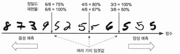
임계값을 오른쪽으로 옮길수록 positive 예측 비율이 높아지므로 precision이 증가한다(recall은 감소한다).
임계값을 왼쪽으로 옮길수록 negative 예측 비율이 높아지므로 recall이 증가한다(precision은 감소한다).

y_scores = sgd_clf.decision_function([some_digit])
y_scores
>> array([2164.22030239])

임계값을 0으로 설정 - true 반환

threshold = 0
y_some_digit_pred = (y_scores > threshold)
y_some_digit_pred
>> array([ True])

임계값을 3000으로 설정 - false 반환
➡ positive로 예측되는 비율이 적어진다고 할 수 있다.

threshold = 3000
y_some_digit_pred = (y_scores > threshold)
y_some_digit_pred
>> array([False])

임계값이 오른쪽으로 이동할수록➡임계값을 높일수록 recall이 감소함을 알 수 있다.
✔ precision과 recall을 동시에 높은 값으로 얻을 수는 없다.

적절한 임계값을 정하는 방법은?
✔ 학습이 완료된 모델에서 임계값을 조절해 조건에 맞는 모델을 찾는다.
- cross_val_predict() 를 이용해 훈련 데이터 셋에 있는 모든 샘플의 점수score를 구한다. (method = "decision_function")
```
y_scores = cross_val_predict(sgd_clf, X_train, y_train_5, cv=3, method="decision_function")
```
- precision_recall_curve() 를 이용해 가능한 모든 임계값에 대해 precision과 recall을 계산하고 그래프로 나타낸다.

precisions, recalls, thresholds = precision_recall_curve(y_train_5, y_scores)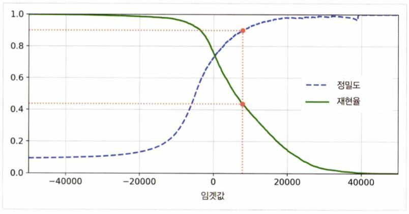

좋은 precision/recall tradeoff를 선택하려면?

재현율에 대한 정밀도 곡선을 그려본다.

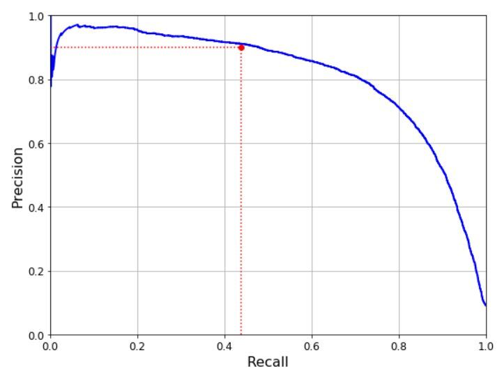
precision이 급격히 떨어지는 지점(80% recall 부근)이 존재한다.
이러한 하강점 직전의 임계값을 선택하는 것이 좋다.

원하는 precision/recall 값이 없을 경우 curve 자체가 변해야 한다.
(○) 더 좋은 모델로 변경 (그래프 자체가 위로 이동한다.)
(△) 더 좋은 parameter 선택/다시 학습

90% precision을 달성하는 지점 찾기

#90% precision을 달성하는 첫번째 인덱스(가장 작은 임계값)
idx_for_90_precision = (precisions >= 0.90).argmax() 
threshold_for_90_precision = thresholds[idx_for_90_precision]
threshold_for_90_precision
>> 3370.0194991439557
#precision 90이 넘는 예측값
y_train_pred_90 = (y_scores >= threshold_for_90_precision)
#precision
precision_score(y_train_5, y_train_pred_90)
>> 0.9000345901072293
#recall
recall_at_90_precision = recall_score(y_train_5, y_train_pred_90)
>> 0.4799852425751706

3.5 ROC Curve

False Positive Rate 에 대한 True Positive Rate(Recall) 곡선

FPR : 실제 negative인 것들 중 positive로 분류된 비율
FP/(FP+TN)
TNR : 실제 negative인 것들 중 negative로 옳게 분류된 비율
TN/(FP+TN) = 특이도(specificity)
FPR = 1 - TNR = 1 - specificity

✔ ROC 곡선 = recall에 대한 (1-특이도) 그래프

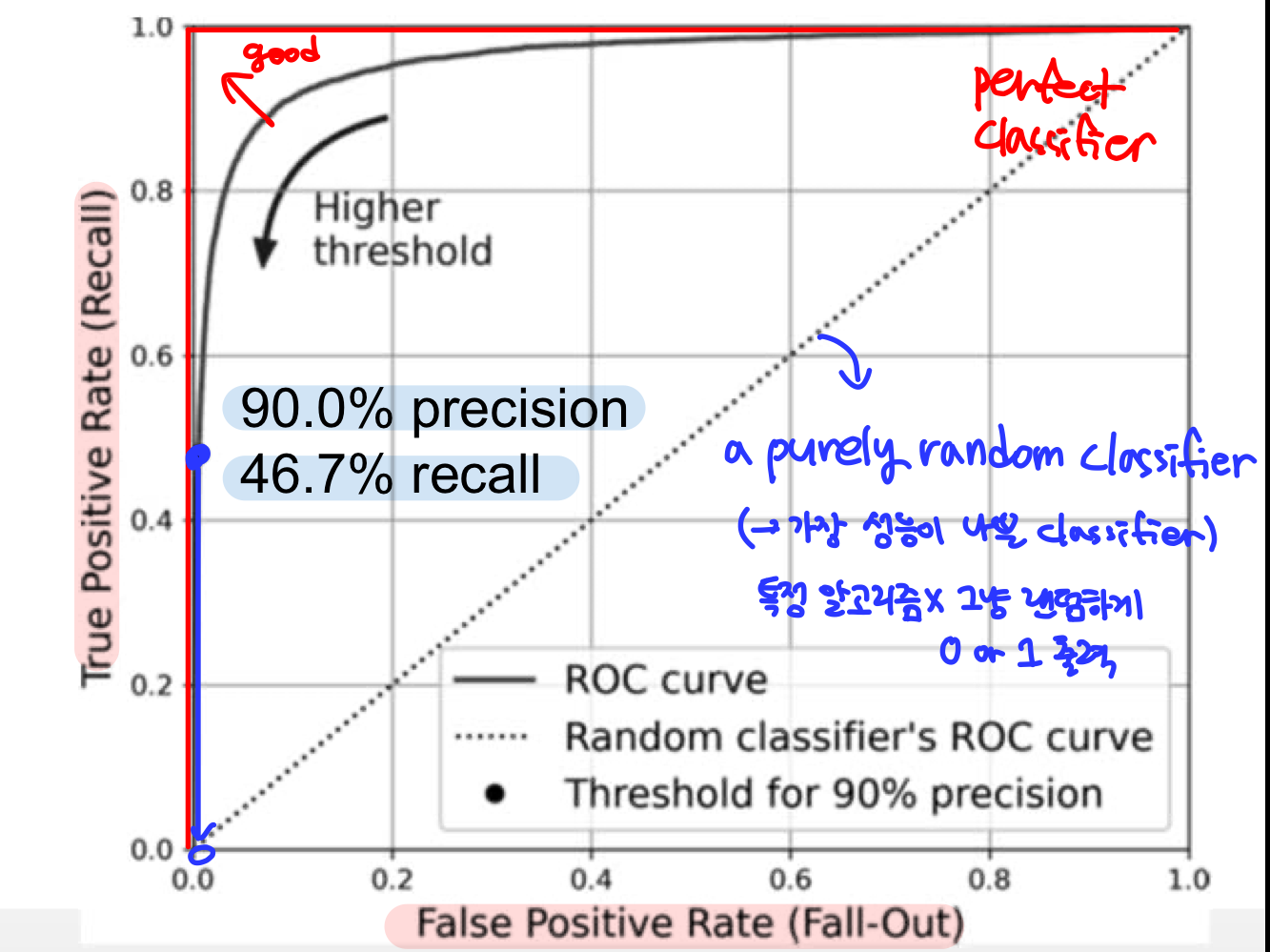
TPR(Recall)과 FPR 모두 positive로 분류된 비율이므로, TPR(Recall)이 높을수록 FPR이 높은 tradeoff가 존재한다.

#fpt, tpr, 임계값을 반환한다.
#매개변수는 레이블(5인 데이터)와 점수
fpr, tpr, thresholds = roc_curve(y_train_5, y_scores)

P/R vs. ROC curve

positive class가 희소하거나 FP가 중요한 경우 P/R curve를 사용한다.
ex) 5-detector : 5(positive) 10% < not 5(negative) 90%

그 외에는 ROC/AUC curve를 사용한다.

✔ 점선 (purely random classifier)에서 멀어질수록 좋은 ROC 곡선이 된다.
➡ 곡선 아래의 면적과 같다고 봐도 무방하다. = AUC

AUC (Area Under the Curve)
: ROC 곡선 아래의 면적을 의미하며, 이 값으로 분류기의 성능을 측정할 수 있다.
AUC = 1 : perfect classifier
AUC = 0.5 : purely random classifier (가장 나쁨)
✔ ROC curve 가 끝점에 가까울수록 좋다 = AUC가 1에 가까울수록 좋다

	from sklearn.metrics import roc_auc_score
	roc_auc_score(y_train_5, y_scores)
	>> 0.9604938554008616

Random forest
predict_proba() 로 점수를 얻는다. ➡ 점수로 확률을 사용함

    from sklearn.ensemble import RandomForestClassifier
	forest_clf = RandomForestClassifier(n_estimators=100, random_state=42)
    
    #이미지가 5일 확률을 반환
    y_probas_forest = cross_val_predict(forest_clf, X_train, y_train_5, cv=3,
                                    method="predict_proba")
    y_probas_forest[:2]
    >> array([[0.11, 0.89],
            [0.99, 0.01]])

predict_proba()

각 class에 해당할 확률을 반환한다.

3개 class인 경우 > [클래스 0일 확률, 클래스 1일 확률, 클래스 2일 확률] 출력

분류 모델에서만 사용 가능(회귀에서는 불가)

	y_scores_forest = y_probas_forest[:, 1] #positive class일 확률 = 5일 확률 저장
    precisions_forest, recalls_forest, thresholds_forest = precision_recall_curve(
    y_train_5, y_scores_forest)
    
    y_train_pred_forest = y_probas_forest[:, 1] >= 0.5  #positive일 확률 ≥ 50%
	f1_score(y_train_5, y_train_pred_forest)
	>> 0.9274509803921569
	roc_auc_score(y_train_5, y_scores_forest)
	>> 0.9983436731328145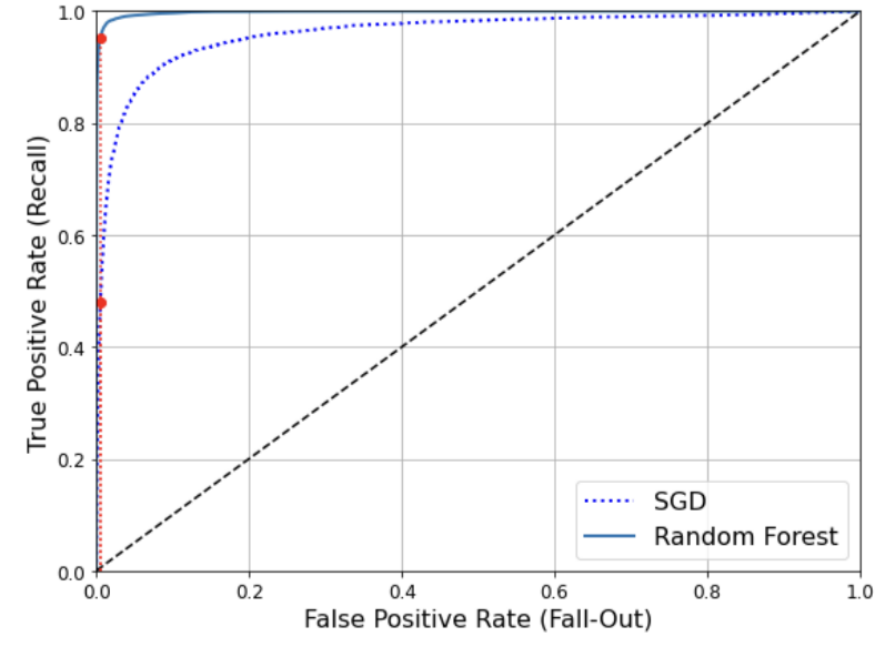

Random Forest가 끝점에 더 가깝다. ➡ AUC 점수가 더 높다.

앙버터

그래도 해야지 어떡해

다음 포스트