사이킷런으로 수행하는 타이타닉 생존자 예측

1. 데이터 확인 및 처리

import numpy as np
import pandas as pd
import matplotlib.pyplot as plt
import seaborn as sns
%matplotlib inline

import warnings
warnings.filterwarnings('ignore')

titanic_df = pd.read_csv('./kaggle/titanic/train.csv')
titanic_df.head(3)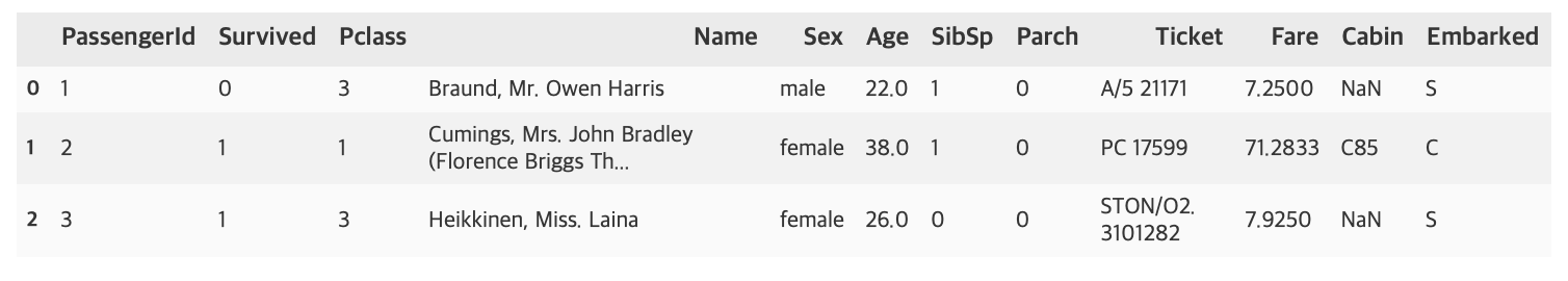

• PassengerId: 탑승자 데이터 일련번호
• Survived: 생존여부, 0 = 사망, 1 = 생존
• Pclass: 티켓의 선실 등급, 1 = 일등석, 2 = 이등석, 3 = 삼등석
• Sex: 탑승자 성별
• Name: 탑승자 이름
• Age: 탑승자 나이
• SibSp: 같이 탑승한 형제, 자매 또는 배우자 인원 수
• Parch: 같이 탑승한 부모님 또는 자녀 인원 수
• Ticket: 티켓 번호
• Fare: 요금
• Cabin: 선실 번호
• Embarked: 탑승 항구, C = Cherbourg, Q = Queenstown, S = Southampton

print(titanic_df.info())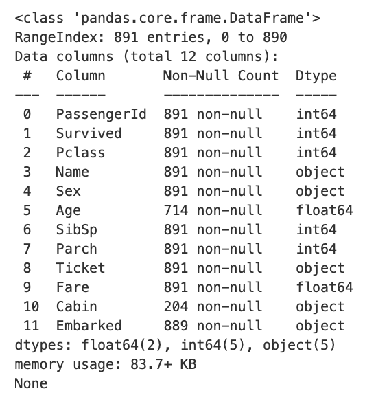

1. 데이터

   • 891개의 로우
   • 12개의 칼럼
   • 2개의 float64 타입
   • 5개의 int64 타입
   • 5개의 object 타입(String 타입으로 봐도 무방함)

2. Null값

   • Age: 177개
   • Cabin: 608개
   • Embarked: 2개

1.1 Null 값 처리

여기서 Age는 평균 나이, 나머지는 "N"으로 Null 값을 채운다.

titanic_df['Age'].fillna(titanic_df['Age'].mean(), inplace=True)
titanic_df['Cabin'].fillna('N', inplace=True)
titanic_df['Embarked'].fillna('N', inplace=True)
print(f'데이터 세트 Null 갯수:\n{titanic_df.isnull().sum()}')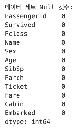

남아있는 문자열 피처 Sex, Cabin, Embarked에 대해 value_counts()를 해보자.

print('Sex 값의 분포:\n',titanic_df['Sex'].value_counts())
print('\nCabin 값의 분포:\n',titanic_df['Cabin'].value_counts())
print('\nEmbarked 값의 분포:\n',titanic_df['Embarked'].value_counts())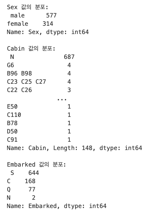

1.2 Cabin 값 추출

Cabin의 선실 번호 중 선실 등급을 나타내는 첫 번째 알파벳이 중요해 보이므로 앞 문자만 추출함.

titanic_df['Cabin'] = titanic_df['Cabin'].str[:1]
print(titanic_df['Cabin'].head())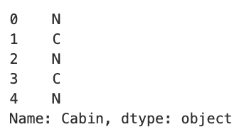

1.3 Sex & Survived

성별에 따른 생존률을 알아보기위해 groupby()와 count()를 사용해보자.

titanic_df.groupby(['Sex', 'Survived'])['Survived'].count()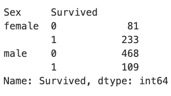

이를 좀 더 보기 편하게 seaborn을 이용해서 시각화를 함.

sns.barplot('Sex', 'Survived', data=titanic_df)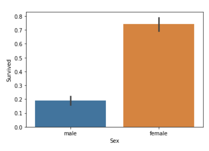

1.4 Pclass, Sex & Survived

이번에는 객실과 성별에 따른 생존률을 알아보겠습니다.

sns.barplot('Pclass', 'Survived', hue='Sex', data=titanic_df)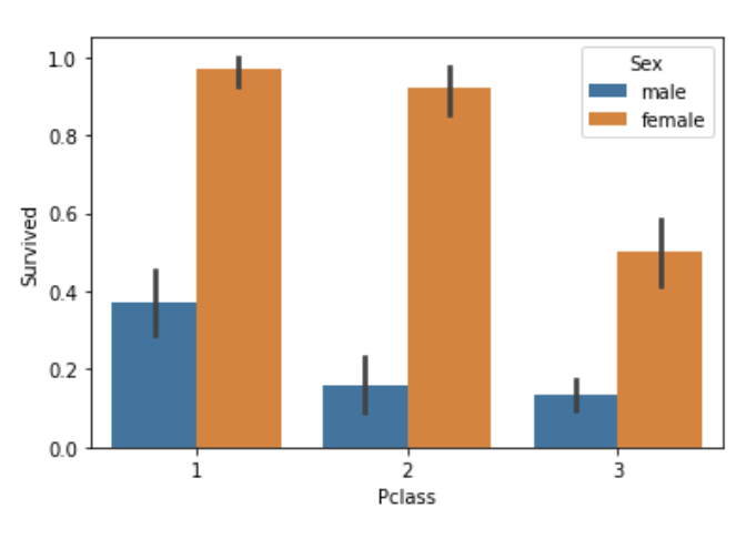

1.5 Age

Pclass가 높은 부자들의 생존률이 더 높고, 남성보다 여성의 생존률이 높은 것을 알 수 있었다.
Age의 경우 값이 너무 다양하기때문에 범위별로 분류해서 카테고리 값을 할당함.

• Baby = 0~5세
• Child = 6~12세
• Teenager = 13~18세
• Student = 19~25세
• Young Adult = 26~35세
• Adult = 36~60세
• Elderly = 61세 이상
• Unknown = -1 이하의 오류 값

def get_category(age):
    cat = ''
    if age <= -1: cat = 'Unknown'
    elif age <= 5: cat = "Baby"
    elif age <= 12: cat = 'Child'
    elif age <= 18: cat = "Teenager"
    elif age <= 25: cat = "Student"
    elif age <= 35: cat = "Young Adult"
    elif age <= 60: cat = "Adult"
    else: cat = 'Elderly'
        
    return cat

plt.figure(figsize=(10, 6))

group_names = ['Unknown', 'Baby', 'Child', 'Teenager', 'Student', 'Young Adult', 'Adult', 'Elderly']

titanic_df['Age_cat'] = titanic_df['Age'].apply(lambda x : get_category(x))
sns.barplot('Age_cat', 'Survived', hue='Sex', data=titanic_df, order=group_names)
titanic_df.drop('Age_cat', axis=1, inplace=True)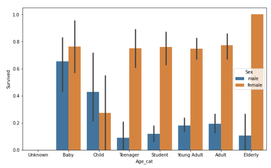

여자 Baby의 경우 생존 확률이 높고 여자 Child의 경우 생존률이 낮은 것으로 나타났다. 그리고 여자 Elderly의 생존률이 매우 높은 것을 알 수 있다. 이제까지 분석한 결과 Sex, Age, Pclass 등이 중요하게 생존을 좌우하는 피처임을 확인할 수 있었다.

1.6 String to Numeric

이제 남아있는 문자열 카테고리 피처를 숫자형 카테고리 피처로 변환해보자.

• 사이킷런의 LabelEncoder 클래스를 사용
• LabelEncoder 객체는 카테고리 값의 유형 수에 따라 0 ~ (카테고리 유형 수 - 1)까지의 숫자 값으로 변환한다.

from sklearn import preprocessing

def encode_features(dataDF):
    features = ['Cabin', 'Sex', 'Embarked']
    for feature in features:
        le = preprocessing.LabelEncoder()
        le = le.fit(dataDF[feature])
        dataDF[feature] = le.transform(dataDF[feature])
    
    return dataDF

titanic_df = encode_features(titanic_df)
titanic_df.head()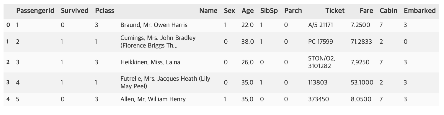

1.7 transform function

지금까지 피처를 가공한 내역을 정리하고 이를 함수로 만들어 쉽게 재사용할 수 있도록 만들어보자. 전처리를 전체적으로 호출하는 함수는 transform_features()이며 Null처리, 포매팅, 인코딩을 수행하는 내부함수로 구성하려한다.

# Null 처리 함수
def fill_na(df):
    df['Age'].fillna(df['Age'].mean(), inplace=True)
    df['Cabin'].fillna('N', inplace=True)
    df['Embarked'].fillna('S', inplace=True)
    df['Fare'].fillna(0, inplace=True)
    
    return df

# 불필요한 칼럼 제거
def drop_features(df):
    df.drop(['PassengerId', 'Name', 'Ticket'], axis=1, inplace=True)
    
    return df

# 레이블 인코딩 수행
def format_features(df):
    df['Cabin'] = df['Cabin'].str[:1]
    features = ['Cabin', 'Sex', 'Embarked']
    for feature in features:
        le = preprocessing.LabelEncoder()
        le = le.fit(df[feature])
        df[feature] = le.transform(df[feature])
    
    return df

# 내부함수 호출
def transform_features(df):
    df = fill_na(df)
    df = drop_features(df)
    df = format_features(df)
    
    return df

2. 사이킷런을 이용한 생존자 예측

만든 함수를 이용해 다시 원본 데이터를 가공해보도록 하자. 원본 CSV 파일을 다시 로딩하고 Survived 속성만 별도로 분리해 클래스 결정값 데이터 세트로 만들고 Survived 속성을 드롭해 피처 데이터 세트로 만든다.

titanic_df = pd.read_csv('./kaggle/titanic/train.csv')
y_titanic_df = titanic_df['Survived']
X_titanic_df = titanic_df.drop('Survived', axis=1)

X_titanic_df = transform_features(X_titanic_df)

from sklearn.model_selection import train_test_split

X_train, X_test, y_train, y_test = train_test_split(X_titanic_df, y_titanic_df, test_size=0.2, random_state=11)

2.1 결정 트리, 랜덤 포레스트, 로지스틱 회귀

결정 트리, 랜덤 포레스트, 로지스틱 회귀를 이용해 타이타닉 생존자를 예측하려 한다. 로지스틱 회귀는 이름은 회귀지만 매우 강력한 분류 알고리즘이다.

from sklearn.tree import DecisionTreeClassifier
from sklearn.ensemble import RandomForestClassifier
from sklearn.linear_model import LogisticRegression
from sklearn.metrics import accuracy_score

dt_clf = DecisionTreeClassifier(random_state=11)
rf_clf = RandomForestClassifier(random_state=11)
lr_clf = LogisticRegression()

# DecisionTreeClassifier 학습/예측/평가
dt_clf.fit(X_train, y_train)
dt_pred = dt_clf.predict(X_test)
print('DecisionTreeClassifier 정확도: {0:.4f}'.format(accuracy_score(y_test, dt_pred)))

# RandomForestClassifier 학습/예측/평가
rf_clf.fit(X_train, y_train)
rf_pred = rf_clf.predict(X_test)
print('RandomForestClassifier 정확도: {0:.4f}'.format(accuracy_score(y_test, rf_pred)))

# LogisticRegression 학습/예측/평가
lr_clf.fit(X_train, y_train)
lr_pred = lr_clf.predict(X_test)
print('LogisticRegression 정확도: {0:.4f}'.format(accuracy_score(y_test, lr_pred)))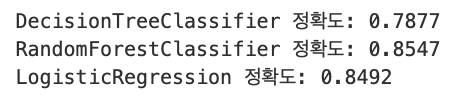

3개의 알고리즘 중 RandomForestClassifier의 정확도가 제일 높게 나오나, 아직 최적화 작업을 수행하지 않았고, 데이터 양도 충분하지 않기 때문에 어떤 알고리즘이 가장 성능이 좋다라고 평가할 수 없다. 그래서 교차검증으로 결정트리를 좀 더 평가해 보려한다.
사이킷런 model_selection 패키지의 KFold 클래스, cross_val_score(), GridSearchCV 클래스를 모두 사용한다.

2.2 결정트리와 K 폴드

# KFold 클래스
from sklearn.model_selection import KFold

def exec_kfold(clf, folds=5):
    # 폴드 세트를 5개인 KFold 객체를 생성, 폴드 수만큼 예측결과 저장을 위한 리스트 객체 생성
    kfold = KFold(n_splits=folds)
    scores = []
    
    # KFold 교차 검증 수행
    for iter_count, (train_index, test_index) in enumerate(kfold.split(X_titanic_df)):
        # X_titanic_df 데이터에서 교차 검증별로 학습과 검증 데이터를 가리키는 index 생성
        X_train, X_test = X_titanic_df.values[train_index], X_titanic_df.values[test_index]
        y_train, y_test = y_titanic_df.values[train_index], y_titanic_df.values[test_index]
        # Classifier 학습, 예측, 정확도 계산
        clf.fit(X_train, y_train)
        predictions = clf.predict(X_test)
        accuracy = accuracy_score(y_test, predictions)
        scores.append(accuracy)
        print('교차 검증 {0} 정확도: {1:.4f}'.format(iter_count, accuracy))
        
    # 5개 fold에서의 평균 정확도 계산
    mean_score = np.mean(scores)
    print('평균 정확도: {0:.4f}'.format(mean_score))

exec_kfold(dt_clf, folds=5)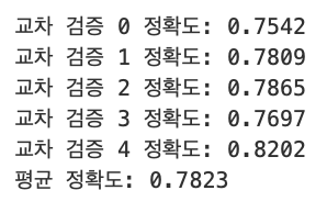

2.3 결정트리와 cross_val_score

# cross_val_score() 클래스
from sklearn.model_selection import cross_val_score

scores = cross_val_score(dt_clf, X_titanic_df, y_titanic_df, cv=5)
for iter_count, accuracy in enumerate(scores):
    print('교차 검증 {0} 정확도: {1:.4}'.format(iter_count, accuracy))
    
print('평균 정확도: {:.4f}'.format(np.mean(scores)))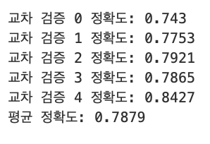

cross_val_score()와 KFold의 평균 정확도가 약간 다른 이유는 cross_val_score()는 StratifiedKFold를 이용해서 폴드 세트를 분할하기 때문이다.

2.4 결정트리와 GridSearchCV

# GridSearchCV() 클래스
from sklearn.model_selection import GridSearchCV

parameters = {'max_depth': [2, 3, 5, 10],
             'min_samples_split': [2, 3, 5],
             'min_samples_leaf': [1, 5, 8]
             }

grid_dclf = GridSearchCV(dt_clf, param_grid=parameters, scoring='accuracy', cv=5)
grid_dclf.fit(X_train, y_train)

print(f'GridSearchCV 최적 하이퍼 파라미터: {grid_dclf.best_params_}')
print(f'GridSearchCV 최고 정확도: {round(grid_dclf.best_score_, 4)}')
best_dclf = grid_dclf.best_estimator_

# GridSearchCV의 최적 하이퍼 파라미터로 학습된 Estimator로 예측 및 평가 수행
dpredictions = best_dclf.predict(X_test)
accuracy = accuracy_score(y_test, dpredictions)
print(f'테스트 세트에서의 DecisionTreeClassifier 정확도: {round(accuracy, 4)}')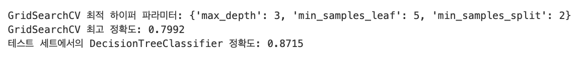

Source: 파이썬 머신러닝 완벽 가이드 / 위키북스