부스팅 개요
부스팅: 여러 개의 약한 학습기 (weak learner)를 순차적으로 학습-예측하면서 잘못 예측한 데이터나 학습 트리에 가중치 부여를 통해 오류를 개선하면서 학습하는 방식
부스팅의 구현 종류
- AdaBoost (Adaptive Boosting)
- Gradient Boost
Gradient Boost는 XGBoost, LightGBM 등이 있음
오리지날 부스팅으로 그냥 GBM (Gradient Boosting Machine)이 있는데 병렬로 학습하는 Random Forest와 다르게 순차적으로 학습을 해서 시간이 좀 오래 걸림
AdaBoost
그림으로 이해해보자
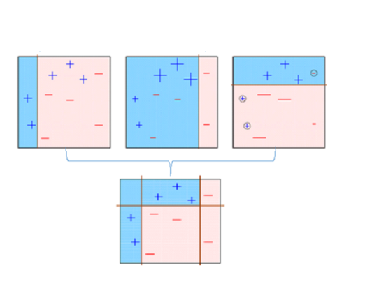
첫 번째 학습기: 세로로 선을 그어서 분류를 진행함 (왼쪽 +, 오른쪽 -)
두 번째 학습기: 첫 번째에서 잘못 분류된 오른쪽 +에 가중치를 주고 적용해서 다시 분류
세 번째 학습기: 두 번째에서 잘못 분류된 것에 가중치를 주고 적용해서 다시 분류
세 가지 약한 학습기를 모두 결합한 것이 최종 학습기
잘 분류된 것을 볼 수 있다!
GBM
GBM (Gradient Boosting Machine): Adaboost와 유사하지만 가중치 업데이트를
경사 하강법 (Gradient Descent)을 이용하는 것이 큰 차이
Gradient Descent
오류 값: 실제 값 - 예측 값
예측 함수를 라고 하면 오류식
이 오류식 를 최소화 하는 방향성을 가지고
반복적으로 가중치 값을 업데이트 하는 것이Gradient Descent
나중에 자세히 다룸
GBM 실습
오리지날 GBM에 대해 실습을 진행해보자
아래처럼 하면 되는데 시간이 너무 오래 걸림
원래도 오래 걸렸는데 scikit-learn이 1.0.x 버전으로 넘어가면서 훨씬 더 걸리는 거 같음
from sklearn.ensemble import GradientBoostingClassifier
import time
import warnings
warnings.filterwarnings('ignore')

X_train, X_test, y_train, y_test = get_human_dataset()

# GBM 수행 시간 측정을 위함. 시작 시간 설정.
start_time = time.time()

gb_clf = GradientBoostingClassifier(random_state=0)
gb_clf.fit(X_train , y_train)
gb_pred = gb_clf.predict(X_test)
gb_accuracy = accuracy_score(y_test, gb_pred)

print('GBM 정확도: {0:.4f}'.format(gb_accuracy))
print("GBM 수행 시간: {0:.1f} 초 ".format(time.time() - start_time))
GBM 정확도: 0.9389
GBM 수행 시간: 580.3 초 시간 찍어보니까 580초가 걸렸음
따라서 그리드 서치는 생략하고 여기서 마무리함
실제로 쓸 일이 없을 것 같음
XGBoost
eXtra Gradient Boost
주요 장점
- 뛰어난 예측 성능
- GBM 대비 빠른 수행 시간 (CPU 병렬 처리, GPU 지원)
- 과적합 방지 (규제 기능 탑재, Tree Pruning)
- 조기 중단 기능, 자체 내장된 교차 검증, 결손값 자체 처리
처음엔 C++로 작성됨 -> 파이썬 Wrapper -> scikit-learn Wrapper
scikt-learn Wrapper는 다른 scikit-learn Estimator들이랑 매우 유사하게 동작 가능
| 항목 | 파이썬 Wrapper | Scikit-learn Wrapper |
|---|---|---|
| 사용 모듈 | import xgboost as xgb | from xgboost import XGBClassifier |
| 데이터세트 활용 | DMatrix 객체 별도 생성 train = xgb.DMatrix(data=X_train, label=y_train) DMatrix 생성자로 Feature 데이터세트와 Label 데이터세트 입력 | NumPy&Pandas 이용 |
| 학습 API | Xgb_model = xgb.train() Xgb_model은 학습된 객체를 반환 받음 | XGBClassifier.fit() |
| 예측 API | xgb.train()으로 학습된 객체에서 predict() 호출 Xgb_model.predict() 반환 결과는 예측 결과가 아니라 예측 결과를 추정하는 확률값 반환 (scikit-learn의 predict_proba()) | XGBClassifier.predict() 예측값 반환 |
| Feature Importance 시각화 | plot_importance() | plot_importance() |
하이퍼 파라미터도 비교해보자
| 파이썬 Wrapper | Scikit-learn Wrapper | 하이퍼 파라미터 설명 |
|---|---|---|
| eta | learning_rate | GBM의 학습률과 같은 파라미터, 0-1 사이 값 지정 부스팅 Step을 반복적으로 수행할 때 업데이트 되는 학습률 값 파이썬 래퍼 디폴트: 0.3, scikit-learn 래퍼 디폴트: 0.1 |
| num_boost_rounds | n_estimators | scikit-learn 앙상블의 n_estimators와 동일, weak learner의 갯수 (반복 수행 횟수) |
| min_child_weight | min_child_weight | 결정 트리의 min_child_leaf와 유사 과적합 조절용 |
| max_depth | max_depth | 결정트리의 max_depth와 동일 트리의 최대 깊이 |
| sub_sample | subsample | GBM의 subsample과 동일 트리가 커져서 과적합 되는 것을 제어하기 위해 데이터를 샘플링하는 비율 sub_sample=0.5면 전체 데이터의 절반을 트리 생성에 사용 0-1사이 값이 가능하지만 일반적으로 0.5-1값 사용 |
| lambda | reg_lambda | L2 규제 적용 값, 디폴트: 1, 값이 클수록 규제 커짐, 과적합 방지 |
| alpha | reg_alpha | L1 규제 적용 값, 디폴트: 0, 값이 클수록 규제 커짐, 과적합 방지 |
| colsample_bytree | colsample_bytree | GBM의 max_feature와 유사 트리 생성에 필요한 Feature(칼럼)을 임의로 샘플링 하는 데 사용 매우 많은 Feature가 있는 경우 과적합 조정에 사용 |
| scale_pos_weight | scale_pos_weight | 특정 값으로 치우치 비대칭한 클래스로 구성된 데이터 세트의 균형을 유지하기 위한 파라미터 디폴트: 1 |
| gamma | gamma | 트리의 리프 노드를 추가적으로 나눌지를 결정할 최소 손실 감소 값 해당 값보다 큰 손실이 감소된 경우 리프 노드를 분리 값이 클수록 과적합 감소 효과 |
scikit-learn Wrapper의 경우 GBM에 동일한 하이퍼 파라미터가 있으면 이를 사용하고, 그렇지 않으면 파이썬 Wrapper의 하이퍼 파라미터 사용
(L1, L2 규제 관한 내용은 회귀에서 다룰 것)
조기 중단 (Early Stopping)
- 계속 학습을 하다 보면 train에 대한 loss를 계속 줄이는 것에 몰두
그것을 방지- 특정 반복 횟수 만큼 더 이상
검증 데이터의 비용함수가 감소하지 않으면 지정된 반복횟수를 다 하지 않고 수행 종료- 학습을 위한 시간 단축, 최적화 튜닝 단계에서 적절히 사용
- 너무 반복 횟수를 줄이면 예측 성능 최적화가 안 된 상태에서 종료 가능성 있으니 주의
- 신경망에서도 많이 씀
- 관련 파라미터:
early_stopping_rounds: 더이상 비용 평가 지표 감소하지 않는 최대 반복 횟수
eval_metric: 반복 수행 시 사용하는 비용 평가 지표
eval_set: 평가 수행하는 별도의 검증 데이터 세트
파이썬 XGBoost 실습
XGboost 실습에는 위스콘신 Breast Cancer 데이터세트 사용
데이터 세트 로딩 후 DataFrame 만들기
import pandas as pd
import numpy as np
from sklearn.datasets import load_breast_cancer
from sklearn.model_selection import train_test_split
# xgboost 패키지 로딩하기
import xgboost as xgb
from xgboost import plot_importance

import warnings
warnings.filterwarnings('ignore')

dataset = load_breast_cancer()
features= dataset.data
labels = dataset.target

cancer_df = pd.DataFrame(data=features, columns=dataset.feature_names)
cancer_df['target']= labels
cancer_df.info()<class 'pandas.core.frame.DataFrame'>
RangeIndex: 569 entries, 0 to 568
Data columns (total 31 columns):
# Column Non-Null Count Dtype
--- ------ -------------- -----
0 mean radius 569 non-null float64
1 mean texture 569 non-null float64
2 mean perimeter 569 non-null float64
3 mean area 569 non-null float64
4 mean smoothness 569 non-null float64
5 mean compactness 569 non-null float64
6 mean concavity 569 non-null float64
7 mean concave points 569 non-null float64
8 mean symmetry 569 non-null float64
9 mean fractal dimension 569 non-null float64
10 radius error 569 non-null float64
11 texture error 569 non-null float64
12 perimeter error 569 non-null float64
13 area error 569 non-null float64
14 smoothness error 569 non-null float64
15 compactness error 569 non-null float64
16 concavity error 569 non-null float64
17 concave points error 569 non-null float64
18 symmetry error 569 non-null float64
19 fractal dimension error 569 non-null float64
20 worst radius 569 non-null float64
21 worst texture 569 non-null float64
22 worst perimeter 569 non-null float64
23 worst area 569 non-null float64
24 worst smoothness 569 non-null float64
25 worst compactness 569 non-null float64
26 worst concavity 569 non-null float64
27 worst concave points 569 non-null float64
28 worst symmetry 569 non-null float64
29 worst fractal dimension 569 non-null float64
30 target 569 non-null int32
dtypes: float64(30), int32(1)
memory usage: 135.7 KBLabel 분포 확인
print(dataset.target_names)
print(cancer_df['target'].value_counts())
['malignant' 'benign'] 1 357 0 212 Name: target, dtype: int64train/test 데이터 세트 분리 후
분리한 train을 다시 train/validation으로 분리
# cancer_df에서 feature용 DataFrame과 Label용 Series 객체 추출
# 맨 마지막 칼럼이 Label이므로 Feature용 DataFrame은 cancer_df의 첫번째 칼럼에서 맨 마지막 두번째 컬럼까지를 :-1 슬라이싱으로 추출.
X_features = cancer_df.iloc[:, :-1]
y_label = cancer_df.iloc[:, -1]

# 전체 데이터 중 80%는 학습용 데이터, 20%는 테스트용 데이터 추출
X_train, X_test, y_train, y_test=train_test_split(X_features, y_label, test_size=0.2, random_state=156 )

# 위에서 만든 X_train, y_train을 다시 쪼개서 90%는 학습과 10%는 검증용 데이터로 분리
X_tr, X_val, y_tr, y_val= train_test_split(X_train, y_train, test_size=0.1, random_state=156 )

print(X_train.shape , X_test.shape)
print(X_tr.shape, X_val.shape)
(455, 30) (114, 30)
(409, 30) (46, 30)각 데이터세트를 DMatrix로 반환
DMatrix는 ndarray, DataFrame에서 모두 반환 가능
파이썬 Wrapper XGBoost에서는 DMatrix를 사용
dtr = xgb.DMatrix(data=X_tr, label=y_tr)
dval = xgb.DMatrix(data=X_val, label=y_val)
dtest = xgb.DMatrix(data=X_test , label=y_test)
하이퍼 파라미터 설정
이진 분류이므로 목적함수(objective): 이진 로지스틱
오류 함수의 성능 평가 지표는 logloss 사용
params = { 'max_depth':3,
           'eta': 0.05,
           'objective':'binary:logistic',
           'eval_metric':'logloss'
        }
num_rounds = 400
주어진 하이퍼 파라미터와 early stopping 파라미터를 train( ) 함수의 파라미터로 전달하고 학습
# 학습 데이터 셋은 'train' 또는 평가 데이터 셋은 'eval' 로 명기
eval_list = [(dtr,'train'),(dval,'eval')] # 또는 eval_list = [(dval,'eval')] 만 명기해도 무방

# 하이퍼 파라미터와 early stopping 파라미터를 train( ) 함수의 파라미터로 전달
xgb_model = xgb.train(params = params , dtrain=dtr , num_boost_round=num_rounds , \
                      early_stopping_rounds=50, evals=eval_list )
[0] train-logloss:0.65016 eval-logloss:0.66183
[1] train-logloss:0.61131 eval-logloss:0.63609
[2] train-logloss:0.57563 eval-logloss:0.61144
[3] train-logloss:0.54310 eval-logloss:0.59204
[4] train-logloss:0.51323 eval-logloss:0.57329
[5] train-logloss:0.48447 eval-logloss:0.55037
[6] train-logloss:0.45796 eval-logloss:0.52929
[7] train-logloss:0.43436 eval-logloss:0.51534
...
[172] train-logloss:0.01297 eval-logloss:0.26157
[173] train-logloss:0.01285 eval-logloss:0.26253
[174] train-logloss:0.01278 eval-logloss:0.26229
[175] train-logloss:0.01267 eval-logloss:0.26086
[176] train-logloss:0.01258 eval-logloss:0.26103
predict()를 통해 예측한 확률 값 반환하고 예측 값으로 변환
파이썬 래퍼에서predict()는 scikit-learn에서predict_proba()와 같다고 생각하면 됨
pred_probs = xgb_model.predict(dtest)
print('predict( ) 수행 결과값을 10개만 표시, 예측 확률 값으로 표시됨')
print(np.round(pred_probs[:10],3))

# 예측 확률이 0.5 보다 크면 1 , 그렇지 않으면 0 으로 예측값 결정하여 List 객체인 preds에 저장
preds = [ 1 if x > 0.5 else 0 for x in pred_probs ]
print('예측값 10개만 표시:',preds[:10])
predict( ) 수행 결과값을 10개만 표시, 예측 확률 값으로 표시됨
[0.845 0.008 0.68 0.081 0.975 0.999 0.998 0.998 0.996 0.001]
예측값 10개만 표시: [1, 0, 1, 0, 1, 1, 1, 1, 1, 0]평가 지표를 출력하는
get_clf_eval()함수 만들어서 예측 평가
from sklearn.metrics import confusion_matrix, accuracy_score
from sklearn.metrics import precision_score, recall_score
from sklearn.metrics import f1_score, roc_auc_score

def get_clf_eval(y_test, pred=None, pred_proba=None):
    confusion = confusion_matrix( y_test, pred)
    accuracy = accuracy_score(y_test , pred)
    precision = precision_score(y_test , pred)
    recall = recall_score(y_test , pred)
    f1 = f1_score(y_test,pred)
    # ROC-AUC 추가
    roc_auc = roc_auc_score(y_test, pred_proba)
    print('오차 행렬')
    print(confusion)
    # ROC-AUC print 추가
    print('정확도: {0:.4f}, 정밀도: {1:.4f}, 재현율: {2:.4f},\
    F1: {3:.4f}, AUC:{4:.4f}'.format(accuracy, precision, recall, f1, roc_auc))

get_clf_eval(y_test , preds, pred_probs)
오차 행렬
[[34 3]
[ 2 75]]
정확도: 0.9561, 정밀도: 0.9615, 재현율: 0.9740, F1: 0.9677, AUC:0.9937Feature Importance 시각화
import matplotlib.pyplot as plt
%matplotlib inline

fig, ax = plt.subplots(figsize=(10, 12))
plot_importance(xgb_model, ax=ax)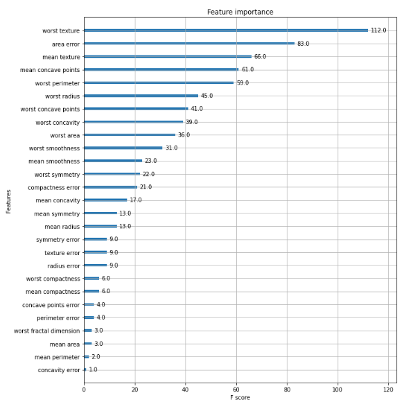
scikit-learn XGBoost 실습
scikit-learn Wrapper import 후 학습과 예측
# 사이킷런 래퍼 XGBoost 클래스인 XGBClassifier 임포트
from xgboost import XGBClassifier

# Warning 메시지를 없애기 위해 eval_metric 값을 XGBClassifier 생성 인자로 입력. 미 입력해도 수행에 문제 없음.
xgb_wrapper = XGBClassifier(n_estimators=400, learning_rate=0.05, max_depth=3, eval_metric='logloss')
xgb_wrapper.fit(X_train, y_train, verbose=True)
w_preds = xgb_wrapper.predict(X_test)
w_pred_proba = xgb_wrapper.predict_proba(X_test)[:, 1]
평가 지표 출력
get_clf_eval(y_test , w_preds, w_pred_proba)오차 행렬
[[34 3]
[ 1 76]]
정확도: 0.9649, 정밀도: 0.9620, 재현율: 0.9870, F1: 0.9744, AUC:0.9954early stopping을 50으로 설정하고 재 학습/예측/평가
from xgboost import XGBClassifier

xgb_wrapper = XGBClassifier(n_estimators=400, learning_rate=0.05, max_depth=3)
evals = [(X_tr, y_tr), (X_val, y_val)]
xgb_wrapper.fit(X_tr, y_tr, early_stopping_rounds=50, eval_metric="logloss",
                eval_set=evals, verbose=True)

ws50_preds = xgb_wrapper.predict(X_test)
ws50_pred_proba = xgb_wrapper.predict_proba(X_test)[:, 1]
[0] validation_0-logloss:0.65016 validation_1-logloss:0.66183
[1] validation_0-logloss:0.61131 validation_1-logloss:0.63609
[2] validation_0-logloss:0.57563 validation_1-logloss:0.61144
[3] validation_0-logloss:0.54310 validation_1-logloss:0.59204
[4] validation_0-logloss:0.51323 validation_1-logloss:0.57329
[5] validation_0-logloss:0.48447 validation_1-logloss:0.55037
[6] validation_0-logloss:0.45796 validation_1-logloss:0.52929
[7] validation_0-logloss:0.43436 validation_1-logloss:0.51534
...
[167] validation_0-logloss:0.01342 validation_1-logloss:0.26203
[168] validation_0-logloss:0.01331 validation_1-logloss:0.26190
[169] validation_0-logloss:0.01319 validation_1-logloss:0.26184
[170] validation_0-logloss:0.01312 validation_1-logloss:0.26133
[171] validation_0-logloss:0.01304 validation_1-logloss:0.26148
[172] validation_0-logloss:0.01297 validation_1-logloss:0.26157
[173] validation_0-logloss:0.01285 validation_1-logloss:0.26253
[174] validation_0-logloss:0.01278 validation_1-logloss:0.26229
[175] validation_0-logloss:0.01267 validation_1-logloss:0.26086get_clf_eval(y_test , ws50_preds, ws50_pred_proba)오차 행렬
[[34 3]
[ 2 75]]
정확도: 0.9561, 정밀도: 0.9615, 재현율: 0.9740, F1: 0.9677, AUC:0.9933지표들이 조금씩 떨어졌는데 원래 early stopping 하면 조금 상승해야 정상
이건 그에 맞는 예제가 아닌 듯
early stopping을 10으로 설정하고 재 학습/예측/평가
# early_stopping_rounds를 10으로 설정하고 재 학습.
xgb_wrapper.fit(X_tr, y_tr, early_stopping_rounds=10,
                eval_metric="logloss", eval_set=evals,verbose=True)

ws10_preds = xgb_wrapper.predict(X_test)
ws10_pred_proba = xgb_wrapper.predict_proba(X_test)[:, 1]
get_clf_eval(y_test , ws10_preds, ws10_pred_proba)
[0]	validation_0-logloss:0.65016	validation_1-logloss:0.66183
[1]	validation_0-logloss:0.61131	validation_1-logloss:0.63609
[2]	validation_0-logloss:0.57563	validation_1-logloss:0.61144
[3]	validation_0-logloss:0.54310	validation_1-logloss:0.59204
[4]	validation_0-logloss:0.51323	validation_1-logloss:0.57329
[5]	validation_0-logloss:0.48447	validation_1-logloss:0.55037
[6]	validation_0-logloss:0.45796	validation_1-logloss:0.52929
[7]	validation_0-logloss:0.43436	validation_1-logloss:0.51534
...
[96]	validation_0-logloss:0.02963	validation_1-logloss:0.26014
[97]	validation_0-logloss:0.02913	validation_1-logloss:0.25974
[98]	validation_0-logloss:0.02866	validation_1-logloss:0.25937
[99]	validation_0-logloss:0.02829	validation_1-logloss:0.25893
[100]	validation_0-logloss:0.02789	validation_1-logloss:0.25928
[101]	validation_0-logloss:0.02751	validation_1-logloss:0.25955
[102]	validation_0-logloss:0.02714	validation_1-logloss:0.25901
오차 행렬
[[34  3]
 [ 3 74]]
정확도: 0.9474, 정밀도: 0.9610, 재현율: 0.9610,    F1: 0.9610, AUC:0.9933
이렇게 너무 일찍 early stoppping 해버리면 성능이 하락할 수 있음
Feature Importance 시각화
from xgboost import plot_importance
import matplotlib.pyplot as plt
%matplotlib inline

fig, ax = plt.subplots(figsize=(10, 12))
# 사이킷런 래퍼 클래스를 입력해도 무방.
plot_importance(xgb_wrapper, ax=ax)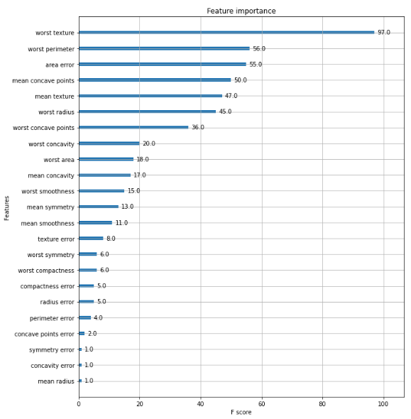
LightGBM
XGBoost 대비 장점
- 더 빠른 학습과 예측 수행 시간
- 더 작은 메모리 사용량
- 카테고리형 피처의 자동 변환과 최적 분할
-> (원-핫 인코딩 등을 사용하지 않고도 카테고리형 피처를 최적으로 변환, 노드 분할 수행)
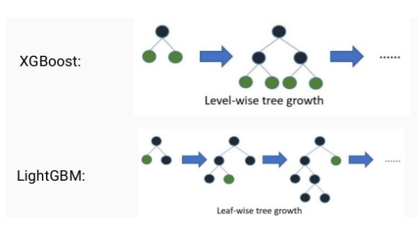
일반적으로 XGBoost를 포함한 GBM 계열은 균형 트리 분할을 함 (depth 최소화)
근데 LightGBM은 리프 중심 트리 분할을 함 (depth 신경 안 씀)
원래 윈도우 기반의 C++로 작성
-> 파이썬 Wrapper
-> scikit-learn Wrapper (LGBMClassifier, LGBMRegressor)
하이퍼 파라미터를 알아보자
| 파이썬 Wrapper | Scikit-learn Wrapper | 하이퍼 파라미터 설명 |
|---|---|---|
| learning_rate | learning_rate | 0-1 사이 값 지정 부스팅 Step을 반복적으로 수행할 때 업데이트 되는 학습률 값 |
| num_iterations | n_estimators | scikit-learn weak learner의 갯수 (반복 수행 횟수) |
| min_data_in_leaf | min_child_samples | 리프 노드가 될 수 있는 최소 데이터 건수(Sample 수) |
| max_depth | max_depth | 결정트리의 max_depth와 동일 트리의 최대 깊이 |
| bagging_fraction | subsample | 트리가 커져서 과적합 되는 것을 제어하기 위해 데이터 샘플링 비율 지정 sub_sample=0.5로 지정하면 전체 데이터의 절반을 트리를 생성하는 데 사용 |
| feature_fraction | colsample_bytree | GBM의 max_feature와 유사 트리 생성에 필요한 Feature를 임의로 샘프링 하는 데 사용 Feature가 너무 많을 경우 과적합 조정 |
| lambda_l2 | reg_lambda | L2 규제 적용 값, 디폴트: 1, 값이 클수록 규제 커짐, 과적합 방지 |
| lambda_l1 | reg_alpha | L1 규제 적용 값, 디폴트: 0, 값이 클수록 규제 커짐, 과적합 방지 |
| early_stopping_round | early_stopping_rounds | 학습 조기 종료를 위한 early stopping interval 값 |
| num_leaves | num_leaves | 최대 리프노드 갯수 |
| min_sum_hessian_in_leaf | min_child_weight | 결정 트리의 min_child_leaf와 유사, 과적합 조절 |
num_leaves의 개수를 중심으로 min_child(samples), max_depth를 함께 조정하면서 모델의 복잡도를 줄이는 것이 기본 튜닝 방안
LightGBM 실습
실습은 scikit-learn Wrapper로 진행함
앞에서 한 scikit-learn XGBoost의 코드와 크게 다르지 않음
마찬가지로 위스콘신 Breast Cancer 데이터세트 이용
# LightGBM의 파이썬 패키지인 lightgbm에서 LGBMClassifier 임포트
from lightgbm import LGBMClassifier

import pandas as pd
import numpy as np
from sklearn.datasets import load_breast_cancer
from sklearn.model_selection import train_test_split
import warnings
warnings.filterwarnings('ignore')

dataset = load_breast_cancer()

cancer_df = pd.DataFrame(data=dataset.data, columns=dataset.feature_names)
cancer_df['target']= dataset.target

cancer_df.info()<class 'pandas.core.frame.DataFrame'>
RangeIndex: 569 entries, 0 to 568
Data columns (total 31 columns):
# Column Non-Null Count Dtype
--- ------ -------------- -----
0 mean radius 569 non-null float64
1 mean texture 569 non-null float64
2 mean perimeter 569 non-null float64
3 mean area 569 non-null float64
4 mean smoothness 569 non-null float64
5 mean compactness 569 non-null float64
6 mean concavity 569 non-null float64
7 mean concave points 569 non-null float64
8 mean symmetry 569 non-null float64
9 mean fractal dimension 569 non-null float64
10 radius error 569 non-null float64
11 texture error 569 non-null float64
12 perimeter error 569 non-null float64
13 area error 569 non-null float64
14 smoothness error 569 non-null float64
15 compactness error 569 non-null float64
16 concavity error 569 non-null float64
17 concave points error 569 non-null float64
18 symmetry error 569 non-null float64
19 fractal dimension error 569 non-null float64
20 worst radius 569 non-null float64
21 worst texture 569 non-null float64
22 worst perimeter 569 non-null float64
23 worst area 569 non-null float64
24 worst smoothness 569 non-null float64
25 worst compactness 569 non-null float64
26 worst concavity 569 non-null float64
27 worst concave points 569 non-null float64
28 worst symmetry 569 non-null float64
29 worst fractal dimension 569 non-null float64
30 target 569 non-null int32
dtypes: float64(30), int32(1)
memory usage: 135.7 KBtrain/validation/test 데이터 분할 후 early stopping까지 진행
X_features = cancer_df.iloc[:, :-1]
y_label = cancer_df.iloc[:, -1]

# 전체 데이터 중 80%는 학습용 데이터, 20%는 테스트용 데이터 추출
X_train, X_test, y_train, y_test=train_test_split(X_features, y_label,
                                         test_size=0.2, random_state=156 )

# 위에서 만든 X_train, y_train을 다시 쪼개서 90%는 학습과 10%는 검증용 데이터로 분리
X_tr, X_val, y_tr, y_val= train_test_split(X_train, y_train,
                                         test_size=0.1, random_state=156 )

# 앞서 XGBoost와 동일하게 n_estimators는 400 설정.
lgbm_wrapper = LGBMClassifier(n_estimators=400, learning_rate=0.05)

# LightGBM도 XGBoost와 동일하게 조기 중단 수행 가능.
evals = [(X_tr, y_tr), (X_val, y_val)]
lgbm_wrapper.fit(X_tr, y_tr, early_stopping_rounds=50, eval_metric="logloss",
                 eval_set=evals, verbose=True)
preds = lgbm_wrapper.predict(X_test)
pred_proba = lgbm_wrapper.predict_proba(X_test)[:, 1]
[1] training's binary_logloss: 0.625671 valid_1's binary_logloss: 0.628248
[2] training's binary_logloss: 0.588173 valid_1's binary_logloss: 0.601106
[3] training's binary_logloss: 0.554518 valid_1's binary_logloss: 0.577587
[4] training's binary_logloss: 0.523972 valid_1's binary_logloss: 0.556324
[5] training's binary_logloss: 0.49615 valid_1's binary_logloss: 0.537407
[6] training's binary_logloss: 0.470108 valid_1's binary_logloss: 0.519401
[7] training's binary_logloss: 0.446647 valid_1's binary_logloss: 0.502637
...
[105] training's binary_logloss: 0.0105953 valid_1's binary_logloss: 0.281454
[106] training's binary_logloss: 0.0102381 valid_1's binary_logloss: 0.282058
[107] training's binary_logloss: 0.00986714 valid_1's binary_logloss: 0.279275
[108] training's binary_logloss: 0.00950998 valid_1's binary_logloss: 0.281427
[109] training's binary_logloss: 0.00915965 valid_1's binary_logloss: 0.280752
[110] training's binary_logloss: 0.00882581 valid_1's binary_logloss: 0.282152
[111] training's binary_logloss: 0.00850714 valid_1's binary_logloss: 0.280894400번 돌리라고 했는데 111에서 끝남
-> 111-50 = 61
61번째loss: 0.2602인데 111번까지 50번 더 돌면서 더 작은 loss를 발견하지 못 함
그래서 그래서 61 + 50 = 111번째에서 멈춘 것
성능 평가 지표 출력
from sklearn.metrics import confusion_matrix, accuracy_score
from sklearn.metrics import precision_score, recall_score
from sklearn.metrics import f1_score, roc_auc_score

def get_clf_eval(y_test, pred=None, pred_proba=None):
    confusion = confusion_matrix( y_test, pred)
    accuracy = accuracy_score(y_test , pred)
    precision = precision_score(y_test , pred)
    recall = recall_score(y_test , pred)
    f1 = f1_score(y_test,pred)
    # ROC-AUC 추가
    roc_auc = roc_auc_score(y_test, pred_proba)
    print('오차 행렬')
    print(confusion)
    # ROC-AUC print 추가
    print('정확도: {0:.4f}, 정밀도: {1:.4f}, 재현율: {2:.4f},\
    F1: {3:.4f}, AUC:{4:.4f}'.format(accuracy, precision, recall, f1, roc_auc))
get_clf_eval(y_test, preds, pred_proba)
오차 행렬
[[34 3]
[ 2 75]]
정확도: 0.9561, 정밀도: 0.9615, 재현율: 0.9740, F1: 0.9677, AUC:0.9877Feature Importance 시각화
# plot_importance( )를 이용하여 feature 중요도 시각화
from lightgbm import plot_importance
import matplotlib.pyplot as plt
%matplotlib inline

fig, ax = plt.subplots(figsize=(10, 12))
plot_importance(lgbm_wrapper, ax=ax)
plt.show()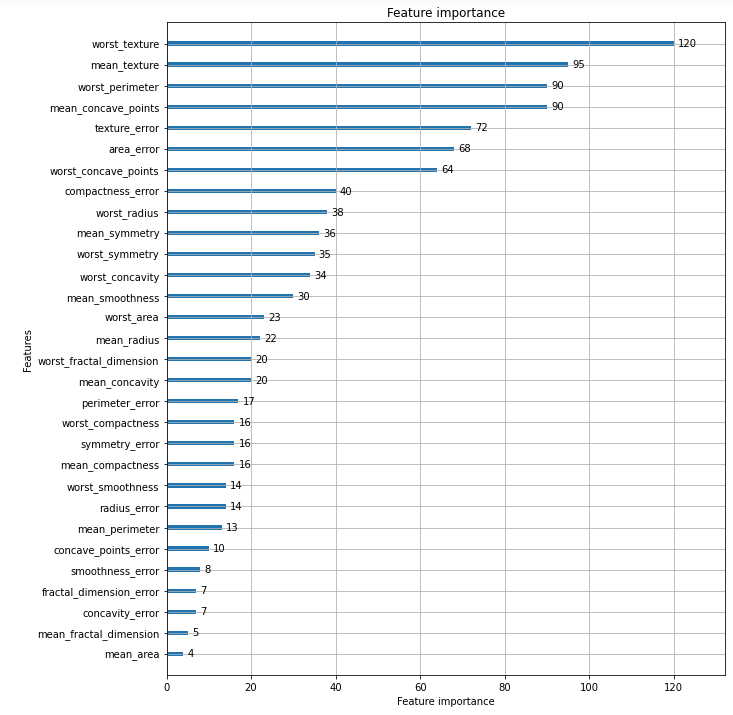
- 일반적으로 데이터 건수가 적으면 XGBoost가 좀 더 높게 나옴
- 요즘 추세는 XGBoost보다 LightGBM을 많이 씀
- 데이터 건수가 많을 때 XGBoost는 너무 오래 걸려서 하이퍼 파라미터 튜닝이 힘듦