회귀 트리 개요
-
scikit-learn의 결정 트리와 결정 트리 기반의 앙상블 알고리즘은 분류 말고 회귀도 가능함
-
트리가 CART (Classification and Regression Tree)를 기반으로 만들어졌기 때문
-
CART 회귀 트리는 분류와 유사하게 분할, 최종 분할이 완료된 후에 각 분할 영역에 있는 데이터 결정값들의 평균 값으로 학습/예측
-
회귀 트리 역시 복잡한 트리 구조를 가질 경우 과적합이 위험이 있고, 트리의 크기와 노드의 개수의 제한 등으로 개선 가능
회귀 트리 실습
scikit-learn의 회귀 트리 클래스 종류
- DecisionTreeRegressor
- GradientBoostingRegressor
- XGBRegressor
- LGBMRegressor
보스톤 집값 예측 데이터 사용
교차 검증까지 진행
from sklearn.datasets import load_boston
from sklearn.model_selection import cross_val_score
from sklearn.ensemble import RandomForestRegressor
import pandas as pd
import numpy as np
import warnings
warnings.filterwarnings('ignore')

# 보스턴 데이터 세트 로드
boston = load_boston()
bostonDF = pd.DataFrame(boston.data, columns = boston.feature_names)

bostonDF['PRICE'] = boston.target
y_target = bostonDF['PRICE']
X_data = bostonDF.drop(['PRICE'], axis=1,inplace=False)

rf = RandomForestRegressor(random_state=0, n_estimators=1000)
neg_mse_scores = cross_val_score(rf, X_data, y_target, scoring="neg_mean_squared_error", cv = 5)
rmse_scores  = np.sqrt(-1 * neg_mse_scores)
avg_rmse = np.mean(rmse_scores)

print(' 5 교차 검증의 개별 Negative MSE scores: ', np.round(neg_mse_scores, 2))
print(' 5 교차 검증의 개별 RMSE scores : ', np.round(rmse_scores, 2))
print(' 5 교차 검증의 평균 RMSE : {0:.3f} '.format(avg_rmse))
5 교차 검증의 개별 Negative MSE scores: [ -7.88 -13.14 -20.57 -46.23 -18.88]
5 교차 검증의 개별 RMSE scores : [2.81 3.63 4.54 6.8 4.34]
5 교차 검증의 평균 RMSE : 4.423 여러 모델로 교차 검증을 하기 위해 함수를 만듦
def get_model_cv_prediction(model, X_data, y_target):
    neg_mse_scores = cross_val_score(model, X_data, y_target, scoring="neg_mean_squared_error", cv = 5)
    rmse_scores  = np.sqrt(-1 * neg_mse_scores)
    avg_rmse = np.mean(rmse_scores)
    print('##### ',model.__class__.__name__ , ' #####')
    print(' 5 교차 검증의 평균 RMSE : {0:.3f} '.format(avg_rmse))
여러 모델 사용해서 평가 수행
#####  DecisionTreeRegressor  #####
 5 교차 검증의 평균 RMSE : 5.978
#####  RandomForestRegressor  #####
 5 교차 검증의 평균 RMSE : 4.423
#####  GradientBoostingRegressor  #####
 5 교차 검증의 평균 RMSE : 4.269
[04:38:41] WARNING: /workspace/src/objective/regression_obj.cu:152: reg:linear is now deprecated in favor of reg:squarederror.
[04:38:41] WARNING: /workspace/src/objective/regression_obj.cu:152: reg:linear is now deprecated in favor of reg:squarederror.
[04:38:42] WARNING: /workspace/src/objective/regression_obj.cu:152: reg:linear is now deprecated in favor of reg:squarederror.
[04:38:42] WARNING: /workspace/src/objective/regression_obj.cu:152: reg:linear is now deprecated in favor of reg:squarederror.
[04:38:43] WARNING: /workspace/src/objective/regression_obj.cu:152: reg:linear is now deprecated in favor of reg:squarederror.
#####  XGBRegressor  #####
 5 교차 검증의 평균 RMSE : 4.089
#####  LGBMRegressor  #####
 5 교차 검증의 평균 RMSE : 4.646
LightGBM이 다 좋은데, 데이터가 작을 경우는 성능이 잘 안 나오는 이슈가 있음
Feature Importance 시각화하기
import seaborn as sns
%matplotlib inline

rf_reg = RandomForestRegressor(n_estimators=1000)

# 앞 예제에서 만들어진 X_data, y_target 데이터 셋을 적용하여 학습합니다.
rf_reg.fit(X_data, y_target)

feature_series = pd.Series(data=rf_reg.feature_importances_, index=X_data.columns)
feature_series = feature_series.sort_values(ascending=False)
sns.barplot(x= feature_series, y=feature_series.index)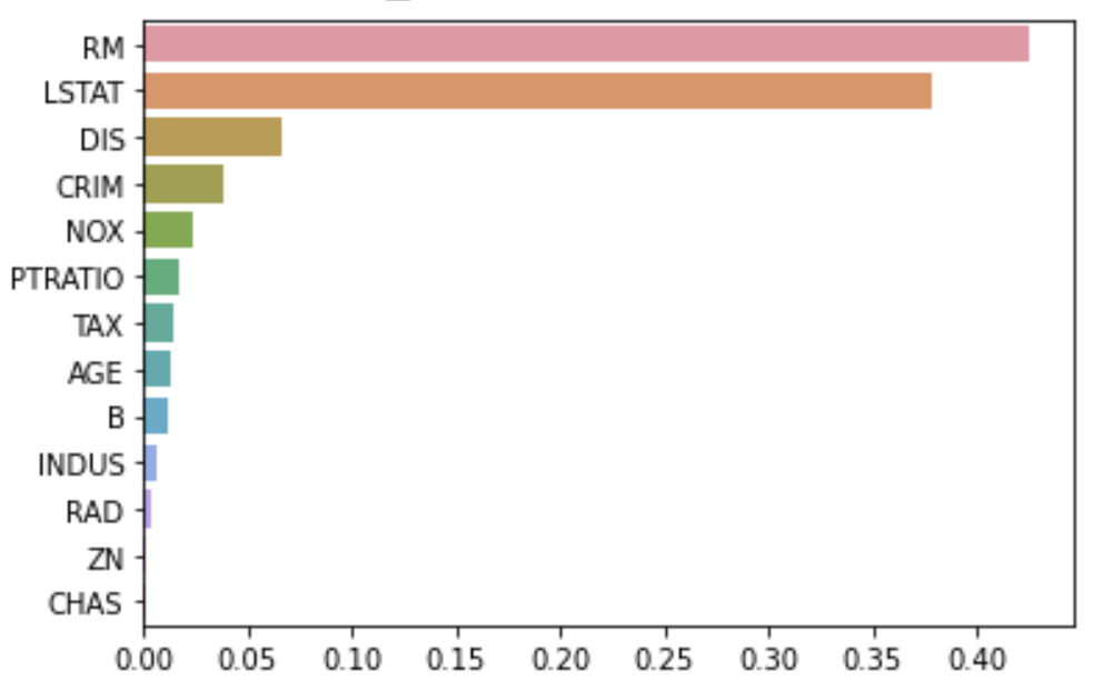
RM과 Label인 PRICE의 상관관계를 보기 위해 산점도 시각화하기
import matplotlib.pyplot as plt
%matplotlib inline

bostonDF_sample = bostonDF[['RM','PRICE']]
bostonDF_sample = bostonDF_sample.sample(n=100,random_state=0)
print(bostonDF_sample.shape)
plt.figure()
plt.scatter(bostonDF_sample.RM , bostonDF_sample.PRICE,c="darkorange")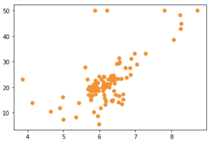
Linear Regression과 max_depth 파라미터를 튜닝한 Decision Tree의 회귀 예측선을 시각화해보자
Feature로는 RM만 사용하고, Lable은 PRICE
import numpy as np
from sklearn.linear_model import LinearRegression

# 선형 회귀와 결정 트리 기반의 Regressor 생성. DecisionTreeRegressor의 max_depth는 각각 2, 7
lr_reg = LinearRegression()
rf_reg2 = DecisionTreeRegressor(max_depth=2)
rf_reg7 = DecisionTreeRegressor(max_depth=7)

# 실제 예측을 적용할 테스트용 데이터 셋을 4.5 ~ 8.5 까지 100개 데이터 셋 생성.
X_test = np.arange(4.5, 8.5, 0.04).reshape(-1, 1)

# 보스턴 주택가격 데이터에서 시각화를 위해 피처는 RM만, 그리고 결정 데이터인 PRICE 추출
X_feature = bostonDF_sample['RM'].values.reshape(-1,1)
y_target = bostonDF_sample['PRICE'].values.reshape(-1,1)

# 학습과 예측 수행.
lr_reg.fit(X_feature, y_target)
rf_reg2.fit(X_feature, y_target)
rf_reg7.fit(X_feature, y_target)

pred_lr = lr_reg.predict(X_test)
pred_rf2 = rf_reg2.predict(X_test)
pred_rf7 = rf_reg7.predict(X_test)
fig , (ax1, ax2, ax3) = plt.subplots(figsize=(14,4), ncols=3)
# X축값을 4.5 ~ 8.5로 변환하며 입력했을 때, 선형 회귀와 결정 트리 회귀 예측 선 시각화
# 선형 회귀로 학습된 모델 회귀 예측선
ax1.set_title('Linear Regression')
ax1.scatter(bostonDF_sample.RM, bostonDF_sample.PRICE, c="darkorange")
ax1.plot(X_test, pred_lr,label="linear", linewidth=2 )
# DecisionTreeRegressor의 max_depth를 2로 했을 때 회귀 예측선
ax2.set_title('Decision Tree Regression: \n max_depth=2')
ax2.scatter(bostonDF_sample.RM, bostonDF_sample.PRICE, c="darkorange")
ax2.plot(X_test, pred_rf2, label="max_depth:2", linewidth=2 )
# DecisionTreeRegressor의 max_depth를 7로 했을 때 회귀 예측선
ax3.set_title('Decision Tree Regression: \n max_depth=7')
ax3.scatter(bostonDF_sample.RM, bostonDF_sample.PRICE, c="darkorange")
ax3.plot(X_test, pred_rf7, label="max_depth:7", linewidth=2)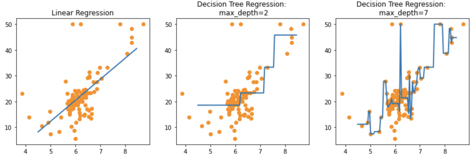
주황색 점은 학습 데이터의 일부, 파란 선은 회귀 예측선임
딱 보니까max_depth=7인 Decision Tree는 과적합 위험 굉장히 높음

Statistics & Data Science