
"날씨정보를 이용해 배추 가격을 예측하기"
특정일의 평균기온, 최저기온, 최대기온, 강수량 데이터가 주어질때, 배추가격을 예측하는 문제 입니다.
-Data set-
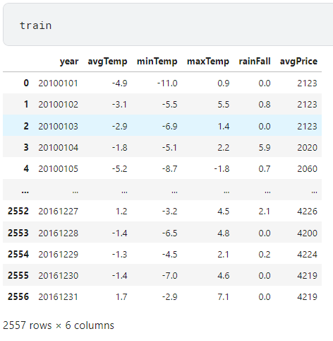
train.csv - 학습용 배추가격 예측을 위한 데이터
▶ year - 년,월,일 정보
▶ avgTemp - 평균기온
▶ minTemp - 최저기온
▶ maxTemp - 최고기온
▶ rainFall - 강수량
▶ avgPrice - 배추가격
test.csv - 평가용 배추가격 예측을 위한 데이터
▶ year - 년,월,일 정보
▶ avgTemp - 평균기온
▶ minTemp - 최저기온
▶ maxTemp - 최고기온
▶ rainFall - 강수량
submit_sample.csv - 평가를 위한 양식
-Code-
Data Load
# This Python 3 environment comes with many helpful analytics libraries installed
# It is defined by the kaggle/python Docker image: https://github.com/kaggle/docker-python
# For example, here's several helpful packages to load

import numpy as np # linear algebra
import pandas as pd # data processing, CSV file I/O (e.g. pd.read_csv)

# Input data files are available in the read-only "../input/" directory
# For example, running this (by clicking run or pressing Shift+Enter) will list all files under the input directory

import os
for dirname, _, filenames in os.walk('/kaggle/input'):
    for filename in filenames:
        print(os.path.join(dirname, filename))

# You can write up to 20GB to the current directory (/kaggle/working/) that gets preserved as output when you create a version using "Save & Run All"
# You can also write temporary files to /kaggle/temp/, but they won't be saved outside of the current session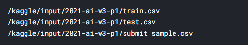
train = pd.read_csv('/kaggle/input/2021-ai-w3-p1/train.csv')
test = pd.read_csv('/kaggle/input/2021-ai-w3-p1/test.csv')
submit_sample = pd.read_csv('/kaggle/input/2021-ai-w3-p1/submit_sample.csv')
Kaggle 대회에 등록되어있는 데이터들을 불러와줍니다.
Data Parsing
year은 모든 행의 개수와 같아 학습에 필요하지 않다고 생각되어 제거 해주었고,
avgPrice는 라벨로 학습되어야 하기 때문에 train에는 제거해주었으며 y_data로 따로 담아주었습니다.
import torch
import torch.optim as optim
data = np.array(train,dtype=np.float64)
data_test = np.array(test,dtype=np.float64)

x_data = data[:, 1:-1]
y_data = data[:, [-1]]
tmp_test = data_test[:, 1:]
x_test = torch.FloatTensor(tmp_test)
x_train = torch.FloatTensor(x_data)
y_train = torch.FloatTensor(y_data)
또한 모든 데이터는 학습에 사용하기 위해 Tensor화 시켜주어 다시 담아주었습니다.
Parameter setting
W = torch.zeros((4,1), requires_grad=True)
b = torch.zeros((1), requires_grad=True)

optimizer = optim.SGD([W,b],lr=0.001)
양배추 가격을 예측하기 위해서 학습에 사용될 데이터는 avgTemp, minTemp, maxTemp, rainFall 총 4개이므로 W는 4행 1열의 0행렬을 만들어주었고 bias또한 0으로 초기화시켜주었습니다.
그리고 requires_grad=True는 이 W와b값이 Gradient Descent계산에 사용된다는 것을 알려주는 코드입니다.
마지막으로 Optimizer는 Gradient Descent방식을 사용하는 SGD방식을 채택했고, learning rate는 0.001로 맞췄습니다.
Training
for step in range(100001):
# H(x) 계산
# Matrix 연산!!
hypothesis = x_train.matmul(W) + b # or .mm or @
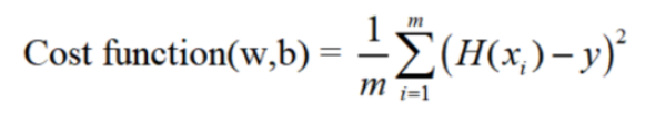
# cost 계산
cost = torch.mean((hypothesis - y_train) ** 2)
# cost로 H(x) 개선
optimizer.zero_grad()
cost.backward()
optimizer.step()
# step번마다 로그 출력
print('#:{} Cost: {:.6f}'.format(
step,cost.item()
))hypothesis = X*W + b 수학적 공식을 코드화 시켜 가설 설정을 하였으며,
아래와 같은 cost function의 수학공식을 코드로 표현해주었습니다.
그다음 optimizer.zero_grad()로 forward를 진행시켜주었고 backward로 cost값을 계산하고 업로드 시켜주었습니다. 마지막으로 Optimizer를 다음 단계로 진행시켜 주는데 이러한 과정을 100000번 시행해 cost가 줄어드는것을 확인 할 수 있었습니다.
#:0 Cost: 12013341.000000
#:1 Cost: 8302531.000000
#:2 Cost: 6246603.500000
#:3 Cost: 5078647.500000
#:4 Cost: 4389976.000000
#:99998 Cost: 1766965.000000
#:99999 Cost: 1766965.000000
#:100000 Cost: 1766965.000000
Predict & Submit
y_pred = x_test.matmul(W) + b
submit_sample['Expected'] = y_pred.detach().numpy()
submit_sample.to_csv('submit_sample.csv', index=False)
지금까지 학습했던 모델의 W값과 test 데이터를 곱하여 다시 값을 도출하게 된다면 test 데이터의 라벨값인 양배추 가격을 예측할 수 있게 됩니다.
예측을 한 값들을 뽑아내어 Tensor로 변환했던 데이터들을 numpy()로 변경해주는 과정을 거쳐 답안지에 담아 제출하여 Baseline점수보다 높은 성능을 보였습니다.