Optimizer없이 경사하강법으로 Linear Regression의 구현하기

이번에는 Gradient Descent 를 optimize 함수를 사용하지 않고 직접 코딩을 통해 구현해볼 것입니다.

▶ Theoretical Overview

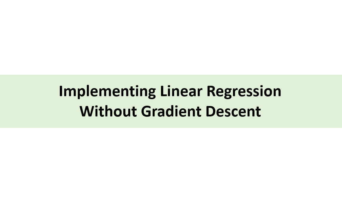
b는 0으로 일단 생략을 하였습니다.

• H(x): 주어진 x 값에 대해 예측을 어떻게 할 것인가
• cost(W): H(x) 가 y 를 얼마나 잘 예측했는가
  Note that it is simplified, without the bias b added to H(x).

▶ Imports

# 시각화용 라이브러리
import matplotlib.pyplot as plt

import numpy as np
import torch
import torch.optim as optim

# For reproducibility
torch.manual_seed(1)

matplotlib.pyplot 시각화 할 때 사용하기 위한 라이브러리입니다.

▶ Data

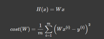
x_train = torch.FloatTensor([[1], [2], [3]])
y_train = torch.FloatTensor([[1], [2], [3]])

# Data
plt.scatter(x_train, y_train)
# Best-fit line
xs = np.linspace(1, 3, 1000)
plt.plot(xs, xs)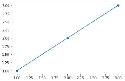

이전 실습과 마찬가지로, x_train과 y_train에 값을 할당해주고, plt라는 라이브러리에서 scatter함수를 활용해 출력을 합니다. numpy의 linspace (Linear Space) 함수를 통해 1에서부터 3까지 1000등분하는 작업을 담아두고, 2D그림을 그리기 위한 plot 함수에 인자값으로 x축 y축으로 설정해주었습니다.

▶ Cost by W

실제로 cost가 어떻게 계산되는지 시각적으로 보기 위해 다음 코드를 작성했습니다.

# -5 ~ 7 사이를 1000등분해서 w_l
# list <= 순차적으로 데이터를 담는 추상자료형

# w_list
W_l = np.linspace(-5, 7, 1000)
# cost list
cost_l = []
for W in W_l:
    hypothesis = W * x_train
    cost = torch.mean((hypothesis - y_train) ** 2)

    cost_l.append(cost.item())
    
    
plt.plot(W_l, cost_l)
plt.xlabel('$W$')
plt.ylabel('Cost')
plt.show()

똑깥이 numpy의 linspace로 -5에서부터 7까지 1000등분한 값을 W_l 에 담았습니다. 그리고 cost 값을 담아둘 cost list를 선언하고 계속 cost 값을 계산하는 반복문을 실행했습니다. 이렇게 담긴 cost와 W값들을 2D 그래프로 나타내는 plot함수로 각각 x축 y축에 설정해주고, 출력해보겠습니다.

x축과 y축의 라벨 즉, 이름을 정해주고 나서 plt.show()를 해줘야 내부적으로 데이터가 도는 것이 아닌 정식으로 Drawing이 되었습니다.

▶ Gradient Descent by Hand

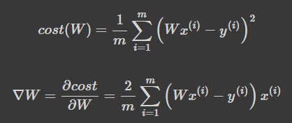
cost 를 W로 편미분하여 gradient 변수에 대입하고 W를 0으로 초기화 하고 위 식을 구현해보겠습니다.

W = 0

# 2/m은 생략 가능
gradient = torch.sum((W * x_train - y_train) * x_train)
print(gradient)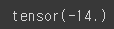

출력을 해보면 cost를 W로 미분한 Gradient값을 구할 수 있게 되는 것입니다.
이제 cost 값을 알 수 있었으니 다음의 W값을 알 수 있습니다.

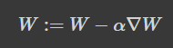
갱신될 W는 현재의 W - lr * cost 의 W로 편미분한 값이 되는 것을 코드로 구현하면,

lr = 0.1
# w = w - lr*gradient
W -= lr * gradient
print(W)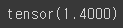

이렇게 W를 갱신해주어 0이었던 W가 1.4가 되었으며 여기까지 직접 코드로 Gradient Descent를 구현하게 되었습니다.

▶ Training

# 데이터
x_train = torch.FloatTensor([[1], [2], [3]])
y_train = torch.FloatTensor([[1], [2], [3]])
# 모델 초기화
W = torch.zeros(1)
# learning rate 설정
lr = 0.1

nb_epochs = 10
for epoch in range(nb_epochs + 1):
    
    # H(x) 계산
    hypothesis = x_train * W
    
    # cost gradient 계산
    cost = torch.mean((hypothesis - y_train) ** 2)
    gradient = torch.sum((W * x_train - y_train) * x_train)

    print('Epoch {:4d}/{} W: {:.3f}, Cost: {:.6f}'.format(
        epoch, nb_epochs, W.item(), cost.item()
    ))

    # cost gradient로 H(x) 개선
    W -= lr * gradient

이렇게 직접 구현한 Gradient descent 알고리즘을 통해 Cost를 계속 줄이고, W를 1에 수렴하도록 만들 수 있었습니다.