Multivariate Linear Regression 구현하기

Linear Regression을 배울 때 Single Linear Regression만 배우는 것이 아니라 x, Feature가 여러개인 Multivatiate Linear Regression을 배워야 합니다.

▶ Theoretical Overview

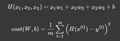
x 변수 하나가 아니라 x_1, x_2 ,x_3 즉, Feature가 여러개인 상황에서 대해서 얘기할 때, 행렬을 도입해서 설명을 해야합니다.

• H(x): 주어진 x 값에 대해 예측을 어떻게 할 것인가
• cost(W,b): H(x) 가 y 를 얼마나 잘 예측했는가

▶ Imports

import torch
import torch.optim as optim

# For reproducibility
torch.manual_seed(1)

라이브러리들을 import하고, seed는 1로 고정시킵니다.

▶ Naive Data Representation

# We will use fake data for this example.

# 데이터
# x1_train == Quiz1 Score , x2_train == Quiz2 Score, x3_train == mid term score
# y_train == Final exam score

x1_train = torch.FloatTensor([[73], [93], [89], [96], [73]])
x2_train = torch.FloatTensor([[80], [88], [91], [98], [66]])
x3_train = torch.FloatTensor([[75], [93], [90], [100], [70]])
y_train = torch.FloatTensor([[152], [185], [180], [196], [142]])

# 모델 초기화
w1 = torch.zeros(1, requires_grad=True)
w2 = torch.zeros(1, requires_grad=True)
w3 = torch.zeros(1, requires_grad=True)
b = torch.zeros(1, requires_grad=True)
# optimizer 설정
optimizer = optim.SGD([w1, w2, w3, b], lr=1e-5)

nb_epochs = 1000
for epoch in range(nb_epochs + 1):
    
    # H(x) 계산
    hypothesis = x1_train * w1 + x2_train * w2 + x3_train * w3 + b

    # cost 계산
    cost = torch.mean((hypothesis - y_train) ** 2)

    # cost로 H(x) 개선
    optimizer.zero_grad()
    cost.backward()
    optimizer.step()

    # 100번마다 로그 출력
    if epoch % 100 == 0:
        print('Epoch {:4d}/{} w1: {:.3f} w2: {:.3f} w3: {:.3f} b: {:.3f} Cost: {:.6f}'.format(
            epoch, nb_epochs, w1.item(), w3.item(), w3.item(), b.item(), cost.item()
        ))

Instance 가 5이고 각각의 Multivariable이 3인 학습용 Data x,y를 설정해주고, 각각의 w와 b를 0으로 초기화하고, 학습용 변수로 선언했습니다. optimizer에는 learning rate인 alpha값을 10의 -5승으로 w1,w2,w3,b를 찾으라는 SGD함수를 통해 Gradient값을 입력받고, cost 계산을 1000번 반복을 하여 출력했습니다.

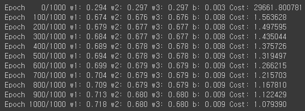
Learning rate가 너무 작아서 w가 갱신되는 값이 미미하게 변화하지만 이 값을 조금 더 키우게 된다면 더 변화되는 값이 두드러지게 보일 것입니다.

▶ Matrix Data Representation

방금 처럼 Naive 하게 하지 않고 Matrix를 통해 이와 같이 정의할 수 있습니다.

x_train = torch.FloatTensor([[73, 80, 75],
                             [93, 88, 93],
                             [89, 91, 90],
                             [96, 98, 100],
                             [73, 66, 70]])
y_train = torch.FloatTensor([[152], [185], [180], [196], [142]])

print(x_train.shape)
print(y_train.shape)

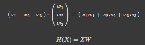
이렇게 행렬로 표기해두면 이전에 하던 것 처럼 w1,w2,w3를 각각 초기화 하고 선언할 필요가 없고, 가설 설정할 때 곱하기 했던 것들이 간단하게 x_train.matmul(w) + b 라는 코를 작성해 Matrix로 계산하게 됩니다.

# 모델 초기화

W = torch.zeros((3, 1), requires_grad=True)
b = torch.zeros(1, requires_grad=True)
# optimizer 설정
optimizer = optim.SGD([W, b], lr=1e-5)

nb_epochs = 20
for epoch in range(nb_epochs + 1):
    
    # H(x) 계산
    # Matrix 연산!!
    hypothesis = x_train.matmul(W) + b # or .mm or @

    # cost 계산
    cost = torch.mean((hypothesis - y_train) ** 2)

    # cost로 H(x) 개선
    # W와 b값 갱신
    optimizer.zero_grad()
    cost.backward()
    optimizer.step()

    # 100번마다 로그 출력
    print('Epoch {:4d}/{} hypothesis: {} Cost: {:.6f}'.format(
        epoch, nb_epochs, hypothesis.squeeze().detach(), cost.item()
    ))

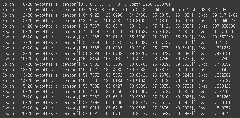
여기까지 실제로 Matirx 연산을 통한 계산과 Matrix가 아닌 Naive 하게 계산하는 방법을 통해서 Multivariate Linear Regression을 Pytorch라는 라이브러리로 구현을 해보았습니다.

이외에 여러가지 영향에 미치는 배추값 예측 문제, 주식 예측 문제같은 것들은 x1,x2,x3라고 하는 Multivariable 로 정의 하고 나서 가설 설정을 하고, 내일의 주식,배추값 등을 예측할 수 있게 될 것 입니다.