[논문 리뷰] Vulnerability-Aware Spatio-Temporal Learning for Generalizable Deepfake Video Detection

1. Introduction

• 기존의 방법 : spatial artifact에 집중 → frame level의 위조에서는 괜찮아도, vedio level에서는 효과가 적음 (spatial + temporal forgery pattern)
• 새로운 방법 : spatial 분기와 temporal 분기로 나눔 → 일반화 능력이 향상됨 → 아래에서 확인하기
• 모델의 최종 결정을 binary classifier 가 전담하는 것은 implicit meaning을 사라지게 함
• regresion temporal branch
  • 특정 지점 - vunerability patch/point == embedding artifacts - 에 집중하는 것이 성능 향상에 도움
• spatial branch
  • spatial 과 temporal domain 간 balance
  • frame-wise temporal spatial artifact 감지
• hand-free ground truth
  • 위의 개념을 구현하기 위해 SBV 모듈 설계
  • 해당 모듈은 HQ 비디오 수준 데이터 합성 알고리즘
• TimeSformer 의 개조
  • 기존 TimeSformer의 경우 temporal, spatial token을 분리함
  • 이 분리한 token을 어떻게 사용하느냐가 논문의 contribution

2. Related Work

1. Video-based Deepfake Detection

• temporal token 과 spatial token 을 같이 봐야 한다.
• 멀리 떨어진 temporal token도 잘 연결돼야 한다.
• 단순 binary classification 만으로는 generalization에 한계가 있다.

2. Data Synthesis

• STC 에서 pseudo-fake를 생성

3. Method

$\mathcal{V} \triangleq \bigcup_{i=1}^{N} \{(X_i, y_i)\}$

• $X_i$ 가 i번째 vedio
• $y_i$ 가 i번째 vedio에 대응하는 T, F label

$\mathcal{V}^r \subset \mathcal{V}$
$\mathcal{\tilde{V}} \triangleq\{ \mathcal{V^r}\cup\mathcal{V^{\tilde{r}}}\}$

• $\mathcal{V}^r$에 속하는 data 에만 의존함
• $\mathcal{V^{\tilde{r}}}$ 은 $\mathcal{V}^r$을 위조한 pseudo-fake data

1. Video-Level Data Synthesis and Augmentation

Self-Blended Video

• 기존의 blending synthesis를 video level에도 확장함
• blending synthesis 가 유효한 전략인가?

의문 1. 실제 deepfake detection dataset에서는 fake가 real 보다 훨씬 많다.

• 논문은, 실제 존재하는 data 분포를 모방하는 것이 아니고, 그럴싸해 보이는 fake 들을 만들어 내면 됨

의문 2. Real-Real blending에서 overfitting?

• 기존 GAN based model 은 위조 흔적이 남는 경우가 다수
• 반면 blending의 경우 mask 위치, noise 강도, 위조 대상이 Random 이므로 통계적으로 랜덤함.
• 또한, spatial artifact가 제거되어 있음
  • 논문에서는 구조적으로 spatial artifact를 보지 못하게 하려고 kernel size를 1로 둠.

결론. 결국 data synthesis가 효과가 있는 이유

• blending data와 1x1 kernel 조합에서 모델이 볼 수 있는 것
  • identity consistency 붕괴 : 눈, 코, 입 간의 어색함
  • semantic inconsistency : 눈, 코, 입의 근육 움직임이 얼굴 전체의 감정 표현과 맞지 않음
  • channel-wise distribution shift : RGB 혹은 채널 별 통계(mean, variance, color tone 등)가 real 데이터와 미묘하게 다름.
  • Frequency statistics mismatch : 고주파, 저주파 에너지 분포가 다름.
  • Global Coherence : 하나의 이미지 안에서 미묘하게 달라지는 조명, 혹은 얼굴의 각도

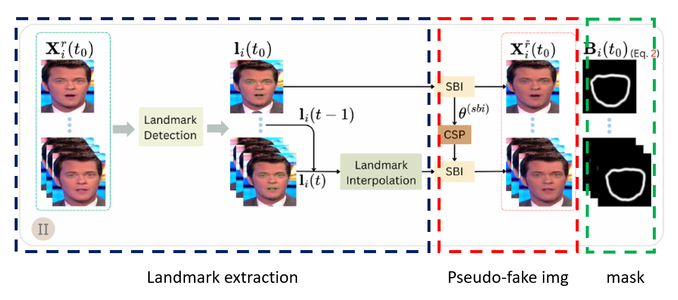
SBV(Self-balanced Video)

1. CSP (consistent synthesized parameters)

• real 비디오의 첫 번째 프레임을 기준으로 랜드마크 점들을 계산한다.
• 그 다음 SBI를 적용해서 pseudo-fake image와 blending mask를 만들고 그것과 관련된 파라미터들을 저장한다. ← 이러면 computing cost가 증가하지 않나..?
• SBI 를 거치면 local artifact가 있을 것으로 예상되는 지점에 대해 마스크가 생성되는 것임
  • 이 마스크는 local artifact를 smoothing함.
• 하지만, SBI만을 사용하면 temporal forgery에는 대비할 수 없음 → 이를 위해 interpolation method 제안
• SBI paper 한 번 쯤 읽어볼 필요가 있음

2. LI (Landmark Inaterpolation module)

$\mathbf{l}_i(t) =\begin{cases} \mathbf{l}_i(t-1) + \frac{\mathbf{l}_i(t) - \mathbf{l}_i(t-1)}{\text{round}(d/\bar{d})}, & \text{if } d > \tau \\ \quad \text{where } d = \left\|\mathbf{l}_i(t) - \mathbf{l}_i(t-1)\right\|_2/n \\ \mathbf{l}_i(t), & \text{otherwise,}\end{cases}$

• 여기서 $\bar{d}$는 어떻게 선택하는 건지 코드상으로 확인 필요
• $\tau$도 얼마인지 코드상으로 확인이 필요
• 이렇게 추출된 마스크에

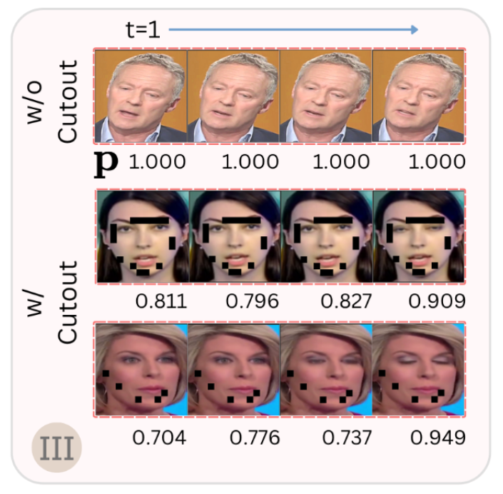
Vulnerability-Driven Cutout Augmentation

• local artifact에 overfitting 되는 것을 방지하는 data augmentation 과정
• local artifact를 masking 후 training
• 아래 과정은 pseudo-fake image가 만들어 지는 과정

$\begin{aligned} \mathbf{B} &= (1 - \mathbf{M}) * \mathbf{M} * 4, \mathbf{B} \in \mathbb{R}^{T \times H \times W}\\ \mathbf{\bar{B}} &= \text{MaxPooling}(\mathbf{B}), \mathbf{\bar{B}} \in \mathbb{R}^{T \times \sqrt{N} \times \sqrt{N}}\\ \mathcal{P} &= \{(l, m)|\bar{B}_{l,m}(t_0) >\tau_{cutout}\} \end{aligned} \rightarrow \mathbf{\tilde B}$

$\mathbf{B}$에서 $\mathbf{\bar{B}}$가 되는 과정

• $\mathbf{B} = (1 - \mathbf{M}) * \mathbf{M} * 4$
  • 여기서 $(1 - \mathbf{M}) * \mathbf{M}$를 하면 마스크 외부와 내부가 맞닿는 경계에서만 값이 생긴다.
  • *4 를 한 것은 scaling효과를 준다.
  • 그 결과 픽셀 레벨에서 경계선에만 1, 나머지는 0에 가까운 값이 주어진다.
• $\mathbf{\bar{B}} = \text{MaxPooling}(\mathbf{B}), \mathbf{\bar{B}} \in \mathbb{R}^{T \times \sqrt{N} \times \sqrt{N}}$
  • 픽셀레벨에서 부여된 값을 maxpooling 한다.
• $\mathcal{P} = \{(l, m)|\bar{B}_{l,m}(t_0) >\tau_{cutout}\}$
  • 위에서 구한 패치를 가지고 임계 이상인 값을 갖는 패치를 마스킹 후보로 정한다.
• 위 과정 전부 코드에서 찾아볼 부분 + N값은 어떻게 정하는지
  

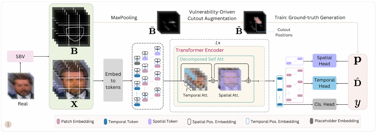
2. FakeSTomer

• temporal artifact를 포착하도록 모델을 설계하자 - 시간 헤드 h, 공간 헤드 g의 도입
• temporal head (h) : blending boundary의 gradiant를 가지고 temporal artifact 탐지
• spatial head (g) : 각 frame 내에서 spatial intensity(artifact) 탐지

1. Backbone : Revisited TimsSformer

• $X \in \mathbb{R}^{C\times T \times H \times W} \rightarrow Z^0 \in \mathbb{R}^{T \times N \times D}$
• 여기서 $X$가 vedio input이고 $Z$가 embedding matrix
• 원래 TimeSformer는 $z_{cls}$가 모든 patch를 사용하여 classification에 이용됨
  • 그러나 이 token은 spatial info와 temporal info를 동시에 본다는 한계가 있음
  • 이를 해결하기 위해 $Z^0 \in \mathbb{R}^{T \times N \times D}$를 도입하고 이 matrix는 temporal token $z_t^0 \in \mathbb{R}^D$와 spatial token $z_s^0 \in \mathbb{R}^D$ 합쳐 놓음
  • 그리고 $z_s^0 \in \mathbb{R}^D$과 $z_t^0 \in \mathbb{R}^D$은 각각 self-attention을 수행함
  • tranfomer 에서 설정한 헤드 개수, 패치 개수 코드상으로 확인
• 이를 한 줄의 수식으로 표현하면 다음과 같다.

$[\mathbf{Z}^L, \mathbf{z}_s^L, \mathbf{z}_t^L] = \Phi(\mathbf{X})$

2. Temporal Haed $h$

• Temporal artifact - temporal high-change - 를 찾자
• $\mathbf{\tilde B}$를 만든 것과 마찬가지로 아래 D를 만든다.
• gradient를 update하는 데 사용한 normalization이 무엇인지 코드상으로 확인이 필요

$\begin{aligned} \mathbf{D} = \frac{\partial \tilde{\mathbf{B}}}{\partial t}, \quad \mathbf{D} \in \mathbb{R}^{T \times \sqrt{N} \times \sqrt{N}} \end{aligned}$

• 해당 gradient를 구하기 위해 regression matrix head를 고안해야 한다.
• Head 는 다음과 같다. 또한 F는 Head에 들어가는 정보이다.
• $\tilde{\mathbf{D}}$는 normalized D 이다.

$\begin{aligned} \mathbf{F} &= \operatorname{Reshape}(\mathbf{Z}^L), \mathbf{F} \in \mathbb{R}^{D \times T \times \sqrt{N} \times \sqrt{N}}\\ \tilde{\mathbf{D}} &= h(\mathbf{F}), \\ h(\cdot) &= \text{3DCnvB}_{3 \times 1 \times 1} \circ \text{3DCnvB}_{3 \times 1 \times 1} \end{aligned}$

• 그 다음 batch norm과 GELU를 거치고 아래 Loss function을 통과한다.

$\mathcal{L}_h = \frac{1}{T \times N} \|\hat{\mathbf{D}} - \tilde{\mathbf{D}}\|_2^2$

• 여기서 새로운 loss function을 만들어 봐도 좋을듯?

3. Spatial Head $g$

• soft label을 사용하도록 한다. → 아마 이 부분에서 overfitting이 더 심한 듯
• pseudo-fake vedio에서 Blending boundary $\mathbf{\tilde B}$를 생성

1. ground truth label 생성

$p(t) = \max_{l,m \in [[1, \sqrt{N}]]} (\tilde{\mathbf{B}}(t))$

• 프레임 안의 모든 spatial patch를 훑고, blending boundary 중 가장 큰 값 하나를 뽑는다.
  • 프레임 안에 blending boundary가 하나라고 있으면 pseudo-fake 영상으로 간주함
  • 만약 blending boundary가 하나도 없다면 0이 됨
  • max값을 줘서, blending boundary가 있냐, 없냐를 민감하게 파악함
• 조금이라도 위치상으로 가짜일 확률이 있는 프레임을 모두 찾아낸다!

2. Architecture Design

$\tilde{\mathbf{p}} = g(\mathbf{z}_s^L) = \mathrm{MLP}(\mathbf{z}_s^L), \tilde{\mathbf{p}} \in \mathbb{R}^T$

3. Objective function

$\mathcal{L}_g = \operatorname{BCE}(\tilde{p}, p)$

4. Training Objective

$\begin{aligned} \tilde{y} &= f(\mathbf{z}_t^L) = \text{MLP}(\mathbf{z}_t^L)\\ \mathcal{L} &= \lambda_c \mathcal{L}_c + \lambda_h \mathcal{L}_h + \lambda_g \mathcal{L}_g \end{aligned}$

• 여기서 말하는 $y$는 dataset에서 제공되는 gt label이다.

3. 정리

• 학습 단계에서는 real-real blending vedion
• test 단계에서는 전체 Deepfake dataset 사용