Canonical Correlation Analysis (CCA)

Introduction

Canonical Correlation Analysis (CCA) is a multivariate statistical method concerned with understanding the relationships between two sets of variables. It was first introduced by Harold Hotelling in the 1930s. CCA seeks to identify and quantify the correlations between linear combinations of the variables in two datasets. The goal is to find pairs of canonical variates—linear combinations of variables within each dataset—that are maximally correlated with each other across the two sets.

Background and Theory

Mathematical Foundations

Consider two sets of variables $X \in \mathbb{R}^{n \times p}$ and $Y \in \mathbb{R}^{n \times q}$, where $n$ is the number of observations, $p$ is the number of variables in the first set, and $q$ is the number of variables in the second set.

CCA seeks to find vectors $a \in \mathbb{R}^{p}$ and $b \in \mathbb{R}^{q}$ such that the correlations between the projections $Xa$ and $Yb$ are maximized. These projections are known as canonical variates.

The correlation coefficient $\rho$ to be maximized is defined as:

The objective is to find $a$ and $b$ that maximize $\rho$.

Optimization Problem

The maximization of $\rho$ can be transformed into an eigenvalue problem. By setting up the Lagrangian for this optimization problem, we obtain the following generalized eigenvalue problems:

where $\lambda$ is the canonical correlation. Solving these eigenvalue problems gives us the canonical coefficients $a$ and $b$ for each pair of canonical variates.

Number of Canonical Correlations

The number of possible pairs of canonical variates is the minimum of $p$ and $q$. However, not all these pairs may be significant. The significance of the canonical correlations can be assessed using statistical tests, such as Bartlett's test of sphericity.

Procedural Steps

1. Preprocessing: Standardize both sets of variables so that each has mean 0 and variance 1.
2. Compute Covariance Matrices: Calculate the covariance matrices $X^T X$, $Y^T Y$, and $X^T Y$.
3. Solve the Eigenvalue Problems: Solve the generalized eigenvalue problems to find the canonical coefficients $a$ and $b$.
4. Calculate Canonical Variates: Compute the canonical variates $Xa$ and $Yb$ for each significant pair of canonical correlations.
5. Assess Significance: Use statistical tests to assess the significance of the canonical correlations.

Implementation

Parameters

• n_components: int Dimensionality of low-space
  

Notes

• CCA requires two distinct datasets X and Y, in which Y is not a target variable.
• Due to its uniqueness in its parameters, CCA may not be compatible with several meta estimators.
• transform() and fit_transform() returns a 2-tuple of Matrix

Examples

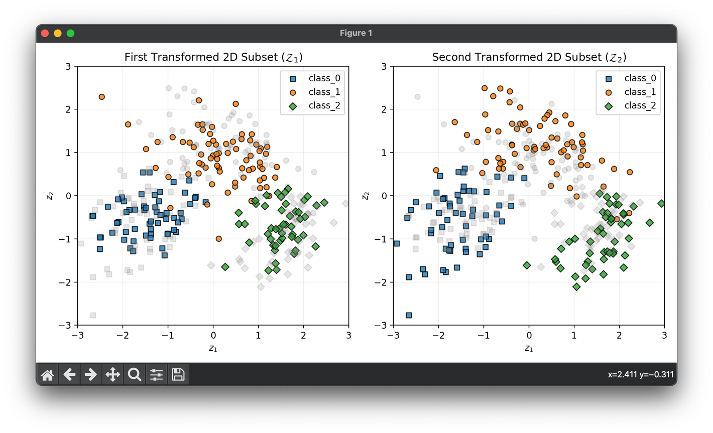
Test with the split wine datasets, each on $\mathbb{R}^6$ and $\mathbb{R}^7$ space respectively:

from luma.reduction.linear import CCA
from luma.preprocessing.scaler import StandardScaler

from sklearn.datasets import load_wine

import matplotlib.pyplot as plt
import numpy as np

data_df = load_wine()
X = data_df.data
y = data_df.target

sc = StandardScaler()
X_std = sc.fit_transform(X)

X1, X2 = X_std[:, :7], X_std[:, 7:]

cca = CCA(n_components=2)
Z1, Z2 = cca.fit_transform(X1, X2)

fig = plt.figure(figsize=(10, 5))
ax1 = fig.add_subplot(1, 2, 1)
ax2 = fig.add_subplot(1, 2, 2)

for cl, lb, m in zip(np.unique(y), data_df.target_names, ["s", "o", "D"]):
    Z1_cl, Z2_cl = Z1[y == cl], Z2[y == cl]
    ax1.scatter(
        Z1_cl[:, 0], 
        Z1_cl[:, 1], 
        label=lb, 
        edgecolors="black", 
        marker=m, 
        alpha=0.8
    )
    ax2.scatter(
        Z2_cl[:, 0], 
        Z2_cl[:, 1], 
        label=lb, 
        edgecolors="black", 
        marker=m, 
        alpha=0.8
    )
    ax1.scatter(Z2_cl[:, 0], Z2_cl[:, 1], color="gray", marker=m, alpha=0.2)
    ax2.scatter(Z1_cl[:, 0], Z1_cl[:, 1], color="gray", marker=m, alpha=0.2)

ax1.set_xlabel(r"$z_1$")
ax1.set_ylabel(r"$z_2$")
ax1.set_title(r"First Transformed 2D Subset ($\mathcal{Z}_1$)")
ax1.set_xlim(-3, 3)
ax1.set_ylim(-3, 3)
ax1.grid(alpha=0.2)
ax1.legend()

ax2.set_xlabel(r"$z_1$")
ax2.set_ylabel(r"$z_2$")
ax2.set_title(r"Second Transformed 2D Subset ($\mathcal{Z}_2$)")
ax2.set_xlim(-3, 3)
ax2.set_ylim(-3, 3)
ax2.grid(alpha=0.2)
ax2.legend()

plt.tight_layout()
plt.show()

Applications

CCA is widely used in various fields, including psychology, where it might be used to understand the relationship between cognitive tests and brain activity patterns; in finance, to discover links between different sets of economic indicators; and in bioinformatics, for integrating different types of genomic data to uncover biological relationships.

Strengths and Limitations

Strengths

• Versatility: CCA can be applied to many types of data and in various fields.
• Insightful: It provides insights into the relationships between sets of variables that might not be apparent from direct correlation analysis.

Limitations

• Data Requirements: Requires large datasets to compute reliable correlations and canonical variates.
• Interpretation Challenges: The interpretation of canonical variates can sometimes be non-intuitive, especially when the original variables are not easily relatable.
• Assumptions: Assumes linear relationships between the sets of variables.

Advanced Topics

• Regularized CCA: For high-dimensional data, regularization techniques can be applied to the canonical coefficients to prevent overfitting.
• Kernel CCA: Extends CCA to nonlinear relationships by applying the kernel method, allowing the analysis of more complex data structures.
• Sparse CCA: Aims to achieve sparse representations of the canonical variates, making the results easier to interpret by selecting only a subset of all available variables.

References

1. Hotelling, H. "Relations Between Two Sets of Variates." Biometrika, vol. 28, no. 3/4, 1936, pp. 321–377.
2. Hardoon, D. R., Szedmak, S., and Shawe-Taylor, J. "Canonical Correlation Analysis: An Overview with Application to Learning Methods." Neural Computation, vol. 16, no. 12, 2004, pp. 2639–2664.
3. Thompson, B. "Canonical Correlation Analysis." Encyclopedia of Statistics in Behavioral Science, 2005.