Kernel Discriminant Analysis (KDA)

Introduction

Kernel Discriminant Analysis (KDA), also known as Kernel Fisher Discriminant Analysis, is an extension of Linear Discriminant Analysis (LDA) that employs kernel methods to find a linear combination of features that best separates two or more classes of data in a high-dimensional space. KDA is particularly effective for nonlinear dimensionality reduction, as it maps the input data into a higher-dimensional feature space where linear discrimination can be applied.

Background and Theory

KDA combines the principles of LDA with kernel methods, allowing for the identification of nonlinear patterns in the data. While LDA seeks to maximize the ratio of between-class variance to within-class variance in the original feature space, KDA performs this optimization in a higher-dimensional feature space defined by a kernel function.

Mathematical Foundations

Given a dataset with $n$ samples $\{\mathbf{x}_i, y_i\}_{i=1}^n$, where $\mathbf{x}_i \in \mathbb{R}^p$ and $y_i$ is the class label of $\mathbf{x}_i$, KDA aims to project the data into a space where classes are maximally separated. This is achieved through a nonlinear mapping $\phi: \mathbb{R}^p \rightarrow \mathcal{F}$, where $\mathcal{F}$ is the high-dimensional feature space.

Kernel Functions

A kernel function $k(\mathbf{x}, \mathbf{x}')$ computes the inner product between two points in the feature space without explicitly performing the mapping $\phi$, i.e.,

Common kernel functions include the polynomial kernel and the Radial Basis Function (RBF) kernel.

Within-Class and Between-Class Scatter in Feature Space

The within-class scatter matrix $S_W$ and between-class scatter matrix $S_B$ in the feature space are defined as:

• Within-Class Scatter Matrix ($\tilde{S}_W$):
  $\tilde{S}_W = \sum_{j=1}^{C} \sum_{i=1}^{n_j} (\phi(\mathbf{x}_i^j) - \tilde{\mu}_j)(\phi(\mathbf{x}_i^j) - \tilde{\mu}_j)^T$
• Between-Class Scatter Matrix ($\tilde{S}_B$):
  $\tilde{S}_B = \sum_{j=1}^{C} n_j (\tilde{\mu}_j - \tilde{\mu})(\tilde{\mu}_j - \tilde{\mu})^T$

where $\tilde{\mu}_j$ is the mean of the mapped samples in class $j$ in the feature space, $\tilde{\mu}$ is the overall mean of the mapped samples, and $n_j$ is the number of samples in class $j$.

Optimization Problem

KDA seeks to maximize the following criterion in the feature space:

This optimization problem can be reformulated in terms of the kernel matrix $K$ and solved as a generalized eigenvalue problem.

Procedural Steps

1. Compute the Kernel Matrix: Calculate the kernel matrix $K$ using the chosen kernel function for all pairs of input data points.
2. Center the Kernel Matrix: Apply centering in the feature space to ensure that the data is centered.
3. Construct Scatter Matrices: Formulate the within-class and between-class scatter matrices in terms of the kernel matrix.
4. Solve the Eigenvalue Problem: Solve for the eigenvalues and eigenvectors of the generalized eigenvalue problem defined by the scatter matrices.
5. Select Principal Components: Choose the eigenvectors associated with the largest eigenvalues as the principal components for dimensionality reduction.

Implementation

Parameters

• n_components: int
  Dimensionality of low-space
  
• deg: int, default = 2
  Degree of polynomial kernel
  
• gamma: float, default = 1.0
  Shape parameter for RBF, sigmoid, Laplacian kernels
  
• coef: float, default = 0.0
  Additional coefficient for polynomial and sigmoid kernels
  
• kernel: KernelUtil.func_type, default = ‘rbf’
  Type of kernel function
  

Examples

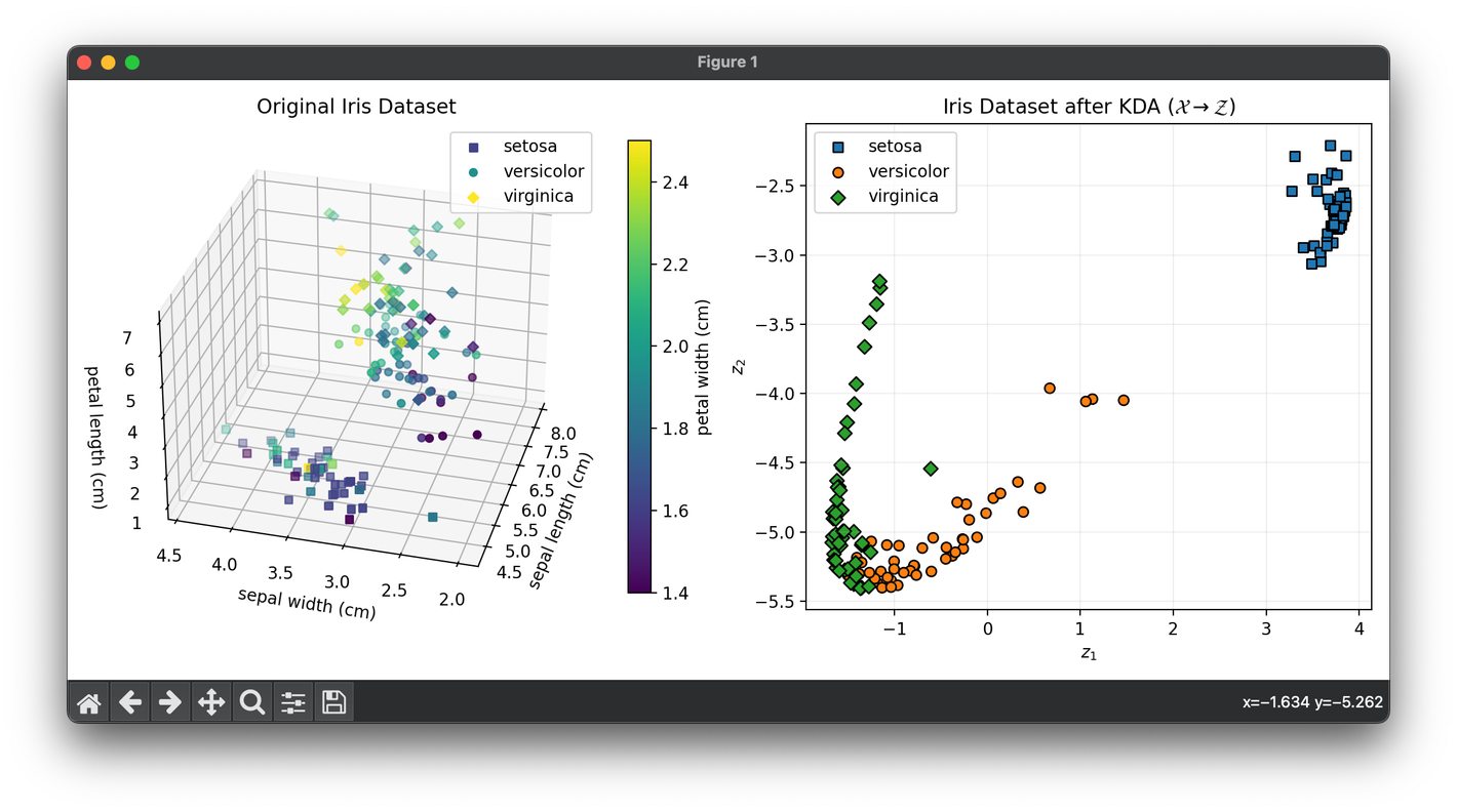
Test on the iris dataset:

from luma.reduction.linear import KDA

from sklearn.datasets import load_iris

import matplotlib.pyplot as plt
import numpy as np

iris_df = load_iris()
X = iris_df.data
y = iris_df.target

model = KDA(n_components=2, gamma=0.1, kernel='rbf')
X_trans = model.fit_transform(X, y)

fig = plt.figure(figsize=(11, 5))
ax1 = fig.add_subplot(1, 2, 1, projection="3d")
ax2 = fig.add_subplot(1, 2, 2)

for cl, m in zip(np.unique(y), ["s", "o", "D"]):
    X_cl = X[y == cl]
    sc = ax1.scatter(
        X_cl[:, 0],
        X_cl[:, 1],
        X_cl[:, 2],
        c=X_cl[:, 3],
        marker=m,
        label=iris_df.target_names[cl],
    )

ax1.set_xlabel(iris_df.feature_names[0])
ax1.set_ylabel(iris_df.feature_names[1])
ax1.set_zlabel(iris_df.feature_names[2])
ax1.set_title("Original Iris Dataset")
ax1.legend()

cbar = ax1.figure.colorbar(sc, fraction=0.04)
cbar.set_label(iris_df.feature_names[3])

for cl, m in zip(np.unique(y), ["s", "o", "D"]):
    X_tr_cl = X_trans[y == cl]
    ax2.scatter(
        X_tr_cl[:, 0],
        X_tr_cl[:, 1],
        marker=m,
        edgecolors="black",
        label=iris_df.target_names[cl],
    )

ax2.set_xlabel(r"$z_1$")
ax2.set_ylabel(r"$z_2$")
ax2.set_title(
    f"Iris Dataset after {type(model).__name__} "
    + r"$(\mathcal{X}\rightarrow\mathcal{Z})$"
)
ax2.legend()
ax2.grid(alpha=0.2)

plt.tight_layout()
plt.show()

Applications

• Nonlinear Dimensionality Reduction: KDA is used to reduce the dimensions of data with nonlinear structures, making it suitable for complex classification tasks.
• Feature Extraction: Extracting features that maximize class separability in a high-dimensional feature space.

Strengths and Limitations

Strengths

• Nonlinear Discrimination: KDA can capture complex, nonlinear relationships between classes.
• Flexibility: The choice of kernel function allows KDA to be adapted to various data structures.

Limitations

• Kernel Selection: The performance of KDA heavily depends on the choice of the kernel function and its parameters.
• Computational Complexity: The need to compute and invert matrices in high-dimensional spaces can be computationally intensive.

References

1. Mika, Sebastian, et al. "Fisher discriminant analysis with kernels." In Neural Networks for Signal Processing IX, 1999. Proceedings of the 1999 IEEE Signal Processing Society Workshop., pp. 41-48. IEEE, 1999.
2. Schölkopf, Bernhard, Alexander Smola, and Klaus-Robert Müller. "Nonlinear component analysis as a kernel eigenvalue problem." Neural computation 10, no. 5 (1998): 1299-1319.
3. Duda, Richard O., Peter E. Hart, and David G. Stork. Pattern Classification. 2nd ed. Wiley-Interscience, 2001.