t-Distributed Stochastic Neighbor Embedding (t-SNE)

Introduction

t-Distributed Stochastic Neighbor Embedding (t-SNE) is a powerful machine learning algorithm for dimensionality reduction, particularly well-suited for the visualization of high-dimensional datasets. It was developed by Laurens van der Maaten and Geoffrey Hinton in 2008. t-SNE excels at capturing the local structure of the data while also revealing clusters or groups within the data, making it an invaluable tool for exploratory data analysis, especially in the fields of bioinformatics, image processing, and natural language processing.

Background and Theory

Dimensionality Reduction

Dimensionality reduction is a process of reducing the number of random variables under consideration, by obtaining a set of principal variables. It can be divided into feature selection and feature extraction. t-SNE falls into the latter category, where the high-dimensional data is transformed into a lower-dimensional space, preserving some property of the original data, typically the pairwise distances between points.

Stochastic Neighbor Embedding (SNE)

The foundation of t-SNE lies in Stochastic Neighbor Embedding (SNE), which converts the high-dimensional Euclidean distances between data points into conditional probabilities that represent similarities.

The similarity of datapoint $x_j$ to datapoint $x_i$ is the conditional probability $p_{j|i}$, that $x_i$ would pick $x_j$ as its neighbor if neighbors were picked in proportion to their probability density under a Gaussian centered at $x_i$.

The conditional probability $p_{j|i}$ is given by:

where $\|x_i - x_j\|^2$ is the squared Euclidean distance between $x_i$ and $x_j$, and $\sigma_i$ is the variance of the Gaussian distribution centered on datapoint $x_i$.

For the low-dimensional counterparts $y_i$ and $y_j$ of the high-dimensional points $x_i$ and $x_j$, the joint probabilities $q_{j|i}$ are computed similarly but using a Student's t-distribution with one degree of freedom (which resembles a Cauchy distribution) to measure similarities:

The t-SNE Algorithm

The t-SNE algorithm minimizes the divergence between two distributions: the distribution that represents the pairwise similarities of the input data points and the distribution that represents the similarities of the corresponding low-dimensional points in the embedding.

The cost function used in t-SNE is the sum of Kullback-Leibler divergences over all datapoints of the joint probabilities $p_{ij}$ and $q_{ij}$, and it is given by:

The minimization of this cost function is typically performed using gradient descent. The gradient of $C$ with respect to the points $y_i$ in the low-dimensional space is:

This formula indicates that points that are close in the high-dimensional space will attract each other in the low-dimensional space, while points that are far apart will repel each other.

Implementation

Parameters

• n_components: int, default = None
  Dimensionality of lower spcae
  
• max_iter: int, default = 1000
  Number of iteration
  
• learning_rate: int, default = 300
  Updating factor of embedding optimization
  
• perplexity: int, default = 30
  Perplexity parameter of Gaussian kernel
  

Examples

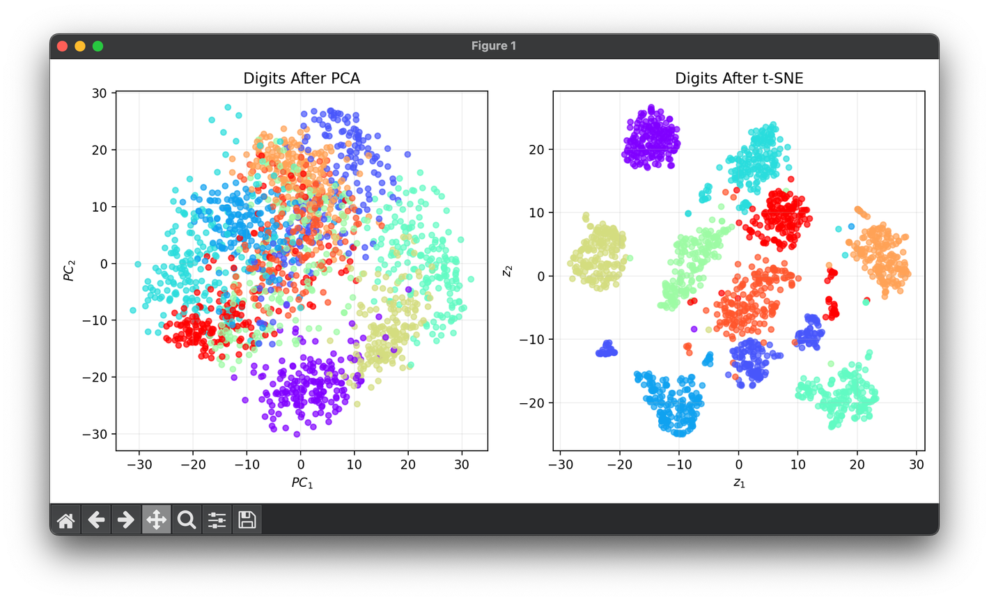
Test on the digits dataset with mapping $\mathbb{R}^{64}\rightarrow\mathbb{R}^2$:

from luma.reduction.manifold import TSNE
from luma.reduction.linear import PCA

from sklearn.datasets import load_digits
import matplotlib.pyplot as plt

X, y = load_digits(return_X_y=True)

pca = PCA(n_components=2)
Z1 = pca.fit_transform(X)

tsne = TSNE(n_components=2,
            max_iter=1000,
            learning_rate=300,
            perplexity=30,
            verbose=True)

Z2 = tsne.fit_transform(X)

fig = plt.figure(figsize=(10, 5))
ax1 = fig.add_subplot(1, 2, 1)
ax2 = fig.add_subplot(1, 2, 2)

ax1.scatter(Z1[:, 0], Z1[:, 1], c=y, cmap='rainbow', s=20, alpha=0.7)
ax1.set_xlabel(r'$PC_1$')
ax1.set_ylabel(r'$PC_2$')
ax1.set_title('Digits After PCA')
ax1.grid(alpha=0.2)

ax2.scatter(Z2[:, 0], Z2[:, 1], c=y, cmap='rainbow', s=20, alpha=0.7)
ax2.set_xlabel(r'$z_1$')
ax2.set_ylabel(r'$z_2$')
ax2.set_title('Digits After t-SNE')
ax2.grid(alpha=0.2)

plt.tight_layout()
plt.show()

Applications

t-SNE has been successfully applied in a wide range of domains including:

• Visualization of high-dimensional data such as genomic data, neural network activations, and datasets with hundreds or thousands of dimensions.
• Clustering and anomaly detection, where the visual separations of data points can indicate the presence of distinct groups or outliers.

Strengths and Limitations

Strengths

• t-SNE is exceptionally good at visualizing clusters or groups within high-dimensional data.
• It can reveal the structure at many scales, providing insights into the data that are not easily observable in the original high-dimensional space.

Limitations

• t-SNE is computationally intensive, especially on large datasets.
• The results of t-SNE are not deterministic; different runs can produce different results due to the random initialization of points.
• Interpreting the distances between clusters in the low-dimensional space can be misleading since t-SNE preserves local structures at the expense of global ones.

Advanced Topics

Parameter Tuning

The choice of perplexity and the learning rate are crucial in determining the quality of the t-SNE embedding. Perplexity can be thought of as a knob that sets the number of effective nearest neighbors. It is typically set between 5 and 50. The learning rate determines how much the positions of points are adjusted during each iteration of the optimization, and it requires some experimentation to find an optimal value.

Variants and Improvements

Several variants and improvements of t-SNE have been proposed, including:

• Accelerated versions of t-SNE that can handle larger datasets more efficiently.
• Techniques to preserve the global structure of the data better, such as UMAP (Uniform Manifold Approximation and Projection).

References

1. van der Maaten, L., & Hinton, G. (2008). Visualizing Data using t-SNE. Journal of Machine Learning Research, 9, 2579-2605.
2. Wattenberg, M., Viégas, F., & Johnson, I. (2016). How to Use t-SNE Effectively. Distill. 🔗