Kernel Principal Component Analysis (KPCA)

Introduction

Kernel Principal Component Analysis (Kernel PCA) is an extension of Principal Component Analysis (PCA) that utilizes kernel methods to perform nonlinear dimensionality reduction. Through the use of kernel functions, Kernel PCA maps the input data into a higher-dimensional feature space where linear PCA is then applied, enabling the capture of nonlinear relationships in the data. This document delves into the conceptual foundation, mathematical underpinnings, and procedural steps of Kernel PCA, aiming to provide a comprehensive understanding suitable for a wide audience.

Background and Theory

Traditional PCA is limited to linear transformations, which can be insufficient for complex, nonlinear data structures. Kernel PCA overcomes this limitation by applying the kernel trick, a method used in support vector machines (SVMs) and other kernel-based algorithms, to implicitly map data to a higher-dimensional space without explicitly computing the coordinates in that space.

Mathematical Foundations

Let $\phi: \mathbb{R}^n \rightarrow \mathcal{F}$ be a nonlinear mapping of the input data $\mathbf{x}$ from its original space $\mathbb{R}^n$ to a higher-dimensional feature space $\mathcal{F}$. The goal of Kernel PCA is to perform PCA in this feature space to exploit the nonlinear structure of the data.

Kernel Functions

A kernel function $k(\mathbf{x}, \mathbf{x}')$ computes the inner product between two points in the feature space $\mathcal{F}$, i.e.,

Common kernel functions include:

• Linear Kernel: $k(\mathbf{x}, \mathbf{x}') = \mathbf{x}^T\mathbf{x}'$
• Polynomial Kernel: $k(\mathbf{x}, \mathbf{x}') = (\gamma \mathbf{x}^T\mathbf{x}' + r)^d$
• Radial Basis Function (RBF) Kernel: $k(\mathbf{x}, \mathbf{x}') = \exp(-\gamma \|\mathbf{x} - \mathbf{x}'\|^2)$

Kernel Matrix (Gram Matrix)

The kernel matrix $K \in \mathbb{R}^{n \times n}$ is defined by computing the kernel function for all pairs of training samples:

Centering in Feature Space

Data must be centered in the feature space. This is achieved by modifying the kernel matrix:

where $1_n$ is an $n \times n$ matrix with all elements equal to $\frac{1}{n}$.

Eigenvalue Problem in Feature Space

Kernel PCA involves solving the eigenvalue problem in the feature space:

The eigenvectors $\mathbf{v}$ of the centered kernel matrix $\tilde{K}$ correspond to the principal components in the feature space.

Procedural Steps

1. Select a Kernel: Choose an appropriate kernel function and its parameters based on the data.
2. Compute the Kernel Matrix: Calculate the kernel matrix $K$ using the chosen kernel function for all pairs of input data points.
3. Center the Kernel Matrix: Apply centering to the kernel matrix to obtain $\tilde{K}$.
4. Solve the Eigenvalue Problem: Compute the eigenvalues and eigenvectors of the centered kernel matrix $\tilde{K}$.
5. Select Principal Components: Choose the leading eigenvectors based on their corresponding eigenvalues. These represent the principal components in the feature space.
6. Project Data: Project the data onto the principal components to achieve dimensionality reduction.

Implementation

Parameters

• n_components: int
  Number of principal components
  
• deg: int, default = 3
  Polynomial degree of polynomial kernel
  
• gamma: float, default = 1.0
  Shape parameter for RBF, sigmoid, Laplacian kernels
  
• coef: float, default = 1.0
  Additional coefficient for polynomial and sigmoid kernels
  
• kernel: KernelUtil.func_type, default = ‘rbf’
  Type of kernel function
  

Examples

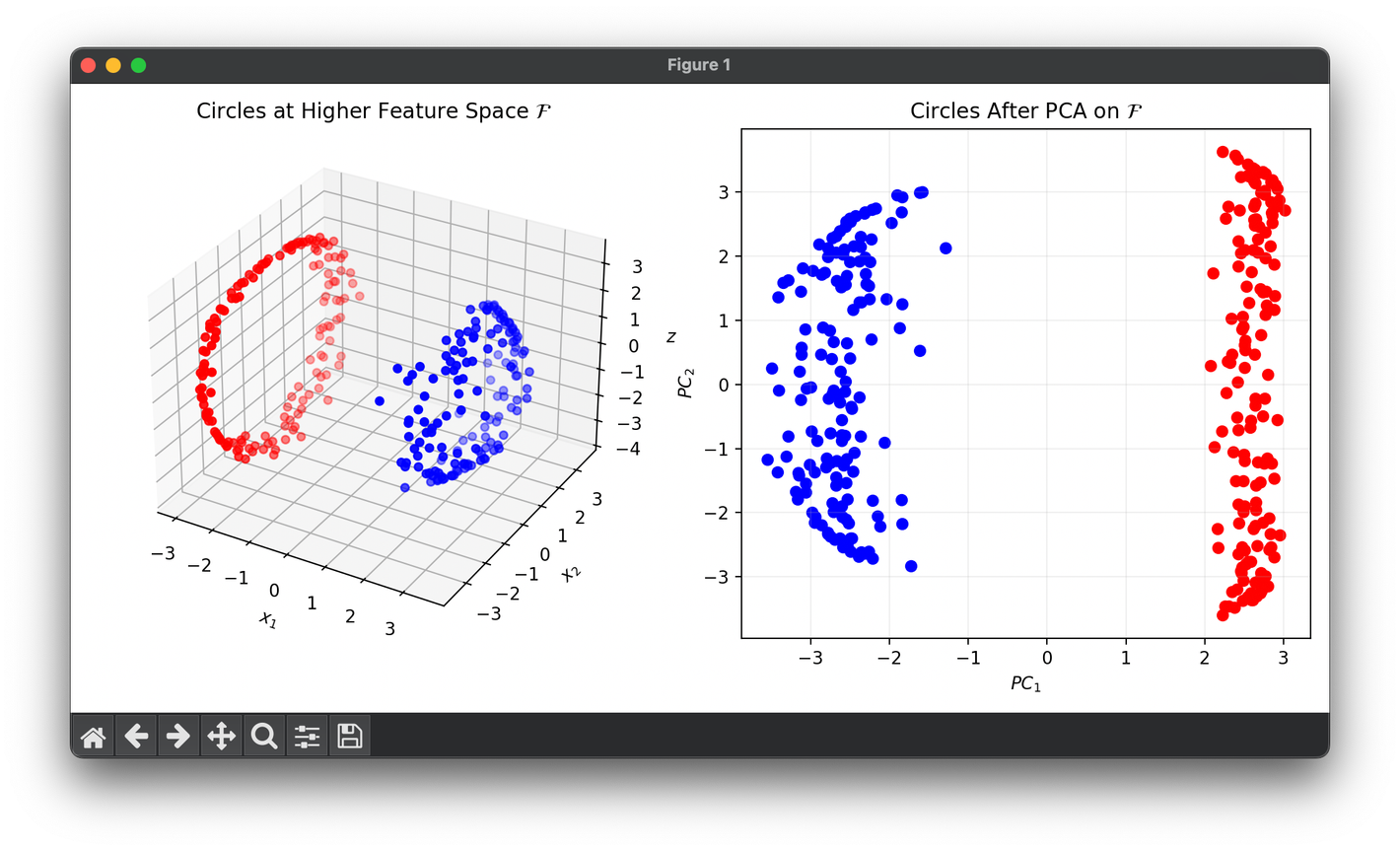
Test with the synthesized two concentric circles dataset:

from luma.reduction.linear import KernelPCA, PCA

from sklearn.datasets import make_circles

import matplotlib.pyplot as plt
import numpy as np

X, y = make_circles(n_samples=300, factor=0.3, noise=0.05, random_state=42)

kpca = KernelPCA(n_components=3, gamma=2.0, kernel="rbf")
pca = PCA(n_components=2)

X_kpca = kpca.fit_transform(X)
X_pca = pca.fit_transform(X_kpca)

fig = plt.figure(figsize=(10, 5))
ax1 = fig.add_subplot(1, 2, 1, projection="3d")
ax2 = fig.add_subplot(1, 2, 2)

for cl, color in zip(np.unique(y), ["r", "b"]):
    X_kpca_cl = X_kpca[y == cl]
    X_pca_cl = X_pca[y == cl]

    ax1.scatter(X_kpca_cl[:, 0], X_kpca_cl[:, 1], X_kpca_cl[:, 2], c=color)
    ax2.scatter(X_pca_cl[:, 0], X_pca_cl[:, 1], c=color)

ax1.set_xlabel(r"$x_1$")
ax1.set_ylabel(r"$x_2$")
ax1.set_zlabel(r"$z$")
ax1.set_title("Circles at Higher Feature Space " + r"$\mathcal{F}$")

ax2.set_xlabel(r"$PC_1$")
ax2.set_ylabel(r"$PC_2$")
ax2.set_title("Circles After PCA on " + r"$\mathcal{F}$")
ax2.grid(alpha=0.2)

plt.tight_layout()
plt.show()

Applications

• Feature Extraction and Dimensionality Reduction: Extracting nonlinear features for machine learning models, especially when linear methods like PCA fall short.
• Data Visualization: Visualizing complex, high-dimensional data in lower-dimensional spaces (e.g., 2D or 3D) for exploratory data analysis.
• Preprocessing: Preparing data for algorithms that benefit from dimensionality reduction, such as clustering and classification tasks.

Strengths and Limitations

Strengths

• Nonlinear Dimensionality Reduction: Capable of uncovering complex, nonlinear structures in the data.
• Flexibility: The choice of kernel allows for customization to specific data characteristics.

Limitations

• Parameter Selection: The performance of Kernel PCA is sensitive to the choice of the kernel function and its parameters.
• Computational Complexity: The requirement to compute and store the kernel matrix can be computationally intensive for large datasets.
• Interpretability: The mapping to a high-dimensional feature space can make the results harder to interpret compared to linear PCA.

Advanced Topics

• Pre-Image Problem: Finding a meaningful representation in the original input space for the data points in the feature space, especially for visualization.
• Incremental Kernel PCA: Techniques for applying Kernel PCA to large datasets or in online settings by incrementally updating the decomposition.

References

1. Schölkopf, Bernhard, Alexander Smola, and Klaus-Robert Müller. "Nonlinear component analysis as a kernel eigenvalue problem." Neural computation 10, no. 5 (1998): 1299-1319.
2. Shawe-Taylor, John, and Nello Cristianini. "Kernel methods for pattern analysis." Cambridge university press, 2004.
3. Bishop, Christopher M. "Pattern Recognition and Machine Learning." Springer, 2006.