Linear Discriminant Analysis (LDA)

Introduction

Linear Discriminant Analysis (LDA) is a supervised machine learning algorithm used for both classification and dimensionality reduction. It seeks to reduce dimensions while preserving as much of the class discriminatory information as possible. Unlike Principal Component Analysis (PCA), which focuses on capturing the variance in the data, LDA aims to model differences between classes. This document provides a comprehensive overview of LDA, focusing on its application in dimensionality reduction, supported by mathematical formulations.

Background and Theory

LDA is based on the concepts of separation and projection. It projects data points onto a lower-dimensional space in a way that maximizes the separability between different classes. This is achieved by maximizing the ratio of the between-class variance to the within-class variance, ensuring that classes are as distinct as possible in the reduced space.

Mathematical Foundations

Consider a dataset with $n$ samples and $p$ features, grouped into $k$ distinct classes. Let $\mathbf{x}_i$ be a sample with class label $y_i$.

Within-Class Scatter Matrix ($S_W$)

The within-class scatter matrix measures the spread of the samples within each class:

where $\mathbf{m}_c$ is the mean vector of class $c$:

and $n_c$ is the number of samples in class $c$.

Between-Class Scatter Matrix ($S_B$)

The between-class scatter matrix measures the spread between the classes:

where $\mathbf{m}$ is the overall mean of the data:

Objective Function

The goal of LDA is to find the projection matrix $\mathbf{W}$ that maximizes the ratio of the determinant of the between-class scatter matrix to the determinant of the within-class scatter matrix in the projected space:

This optimization problem can be solved as a generalized eigenvalue problem:

where $\mathbf{w}$ are the columns of $\mathbf{W}$, the directions to project the data.

Procedural Steps

1. Compute Mean Vectors: Calculate the mean vectors for each class.
2. Compute Scatter Matrices: Calculate the within-class and between-class scatter matrices.
3. Solve the Eigenvalue Problem: Solve for the eigenvalues and eigenvectors of $S_W^{-1}S_B$.
4. Select Linear Discriminants: Choose the top eigenvectors based on their corresponding eigenvalues to form the transformation matrix $\mathbf{W}$.
5. Project Data: Use $\mathbf{W}$ to project the data onto a lower-dimensional space.

Implementation

Parameters

• n_components: int
  Number of linear discriminants
  

Notes

To use LDA for classification, refer to luma.classifier.discriminant.LDAClassifier.

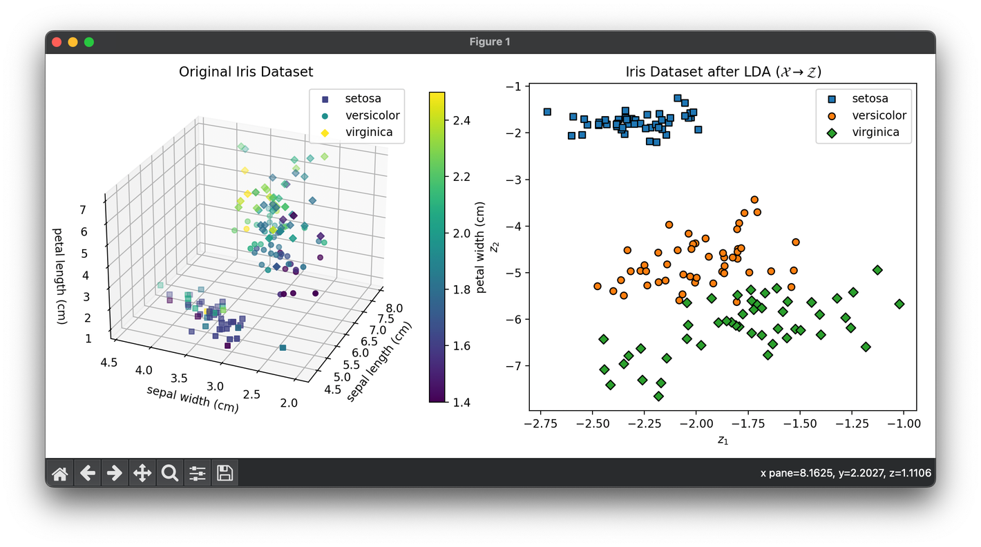
Examples

from luma.reduction.linear import LDA

from sklearn.datasets import load_iris

import matplotlib.pyplot as plt
import numpy as np

iris_df = load_iris()
X = iris_df.data
y = iris_df.target

model = LDA(n_components=2)
X_trans = model.fit_transform(X, y)

fig = plt.figure(figsize=(11, 5))
ax1 = fig.add_subplot(1, 2, 1, projection="3d")
ax2 = fig.add_subplot(1, 2, 2)

for cl, m in zip(np.unique(y), ["s", "o", "D"]):
    X_cl = X[y == cl]
    sc = ax1.scatter(
        X_cl[:, 0],
        X_cl[:, 1],
        X_cl[:, 2],
        c=X_cl[:, 3],
        marker=m,
        label=iris_df.target_names[cl],
    )

ax1.set_xlabel(iris_df.feature_names[0])
ax1.set_ylabel(iris_df.feature_names[1])
ax1.set_zlabel(iris_df.feature_names[2])
ax1.set_title("Original Iris Dataset")
ax1.legend()

cbar = ax1.figure.colorbar(sc, fraction=0.04)
cbar.set_label(iris_df.feature_names[3])

for cl, m in zip(np.unique(y), ["s", "o", "D"]):
    X_tr_cl = X_trans[y == cl]
    ax2.scatter(
        X_tr_cl[:, 0],
        X_tr_cl[:, 1],
        marker=m,
        edgecolors="black",
        label=iris_df.target_names[cl],
    )

ax2.set_xlabel(r"$z_1$")
ax2.set_ylabel(r"$z_2$")
ax2.set_title(
    f"Iris Dataset after {type(model).__name__} "
    + r"$(\mathcal{X}\rightarrow\mathcal{Z})$"
)
ax2.legend()

plt.tight_layout()
plt.show()

Applications

• Feature Extraction: Reducing the dimensionality of input features while maintaining the class-discriminatory information.
• Data Visualization: Projecting data into two or three dimensions for visualization purposes.
• Preprocessing for Classification: Improving the performance of classifiers by reducing the dimensionality of the feature space.

Strengths and Limitations

Strengths

• Class Separation: Explicitly focuses on maximizing class separability.
• Efficiency: Generally requires fewer dimensions to achieve high class separation.

Limitations

• Assumption of Linearity: Assumes linear relationships between features.
• Normal Distribution: Assumes features are normally distributed within each class.
• Equal Covariance: Assumes identical covariance matrices for all classes.

Advanced Topics

• Regularized LDA: Introduces regularization to handle scenarios where $S_W$ is singular or near-singular.
• Kernel LDA: Extends LDA to nonlinear transformations using kernel methods.

References

1. Fisher, R.A. "The use of multiple measurements in taxonomic problems." Annual Eugenics, 7(2):179-188, 1936.
2. Duda, R.O., Hart, P.E., and Stork, D.G. "Pattern Classification." 2nd ed. Wiley-Interscience, 2001.
3. McLachlan, Geoffrey J. "Discriminant Analysis and Statistical Pattern Recognition." Wiley-Interscience, 2004.