Modified Locally Linear Embedding (MLLE)

Introduction

Modified Locally Linear Embedding (MLLE) is an enhanced version of the classic Locally Linear Embedding (LLE) algorithm, designed to address some of its limitations, particularly in preserving the local geometry of the data manifold more accurately. MLLE modifies the standard LLE by using multiple weight vectors to reconstruct each point, aiming to reduce the collapse of reconstructed points into a lower-dimensional space—a phenomenon often seen with LLE.

Background and Theory

LLE is a powerful technique for dimensionality reduction and manifold learning, but it can sometimes suffer from issues like insufficient weight distribution and the tendency for the embedding to collapse. MLLE addresses these problems by employing an improved method for computing the reconstruction weights, resulting in a more stable and accurate embedding that better preserves the local structure of the data manifold.

Mathematical Foundations

Given a dataset $\{ \mathbf{x}_1, \mathbf{x}_2, \ldots, \mathbf{x}_N \}$ where each $\mathbf{x}_i \in \mathbb{R}^D$, MLLE seeks a low-dimensional representation $\{ \mathbf{y}_1, \mathbf{y}_2, \ldots, \mathbf{y}_N \}$ in $\mathbb{R}^d$ ($d < D$), similar to LLE. However, the reconstruction weights in MLLE are computed differently to better capture the local data geometry.

Reconstruction Weights

The key innovation of MLLE is in computing the reconstruction weights. Instead of finding a single weight vector for each point, MLLE calculates multiple weight vectors that reflect different local linear approximations, and then it combines them to form a single, more robust set of weights. This process involves minimizing a modified cost function that takes into account the variance in the local linear approximations, leading to an optimization problem formulated as:

where $\text{Var}(W_{ij})$ represents the variance of the weights associated with the $j$-th neighbor of the $i$-th point, and $\alpha$ is a regularization parameter that controls the trade-off between the fidelity of the reconstruction and the stability of the weights.

Embedding

After computing the reconstruction weights, MLLE finds the low-dimensional embeddings $\mathbf{y}_i$ by minimizing a similar cost function as LLE, aiming to preserve the local configurations dictated by the weights:

with the weights $W_{ij}$ derived from the modified reconstruction process.

Procedural Steps

1. Neighbor Selection: Identify the $K$ nearest neighbors for each data point $\mathbf{x}_i$.
2. Weight Matrix Construction: Compute the reconstruction weights $W_{ij}$ by solving the modified optimization problem that accounts for variance in the local linear approximations.
3. Low-Dimensional Embedding: Calculate the low-dimensional points $\mathbf{y}_i$ that best preserve the local geometric properties, using the computed weights.

Implementation

Parameters

• n_components: int, default = None
  Dimensionality of the lower-dimensional space
  
• n_neighbors: int, default = 5
  Number of neighbors to be considered 'close’
  
• regularization: float, default = 0.001
  Regularization parameter for stability
  

Examples

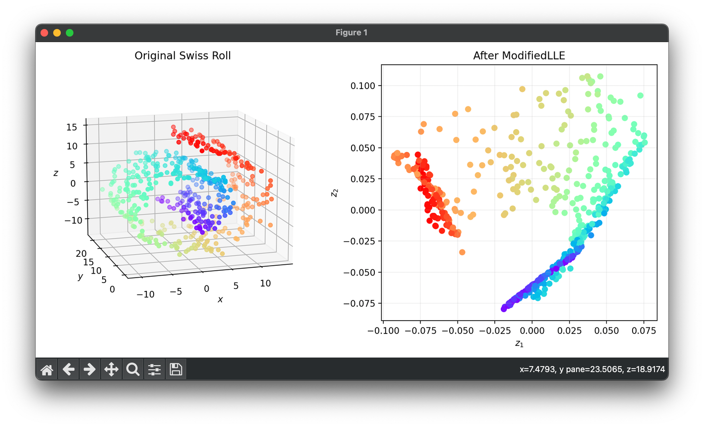
Test on the 3D Swiss roll dataset:

from luma.reduction.manifold import ModifiedLLE

from sklearn.datasets import make_swiss_roll
import matplotlib.pyplot as plt

X, y = make_swiss_roll(n_samples=500, noise=0.5)

model = ModifiedLLE(n_components=2, n_neighbors=7, regularization=1e-3)
Z = model.fit_transform(X)

fig = plt.figure(figsize=(10, 5))
ax1 = fig.add_subplot(1, 2, 1, projection='3d')
ax2 = fig.add_subplot(1, 2, 2)

ax1.scatter(X[:, 0], X[:, 1], X[:, 2], c=y, cmap='rainbow')
ax1.set_xlabel(r'$x$')
ax1.set_ylabel(r'$y$')
ax1.set_zlabel(r'$z$')
ax1.set_title('Original Swiss Roll')

ax2.scatter(Z[:, 0], Z[:, 1], c=y, cmap='rainbow')
ax2.set_xlabel(r'$z_1$')
ax2.set_ylabel(r'$z_2$')
ax2.set_title(f'After {type(model).__name__}')
ax2.grid(alpha=0.2)

plt.tight_layout()
plt.show()

Applications

MLLE is applied in fields requiring dimensionality reduction and manifold learning, like image processing, bioinformatics, and pattern recognition, where preserving the intrinsic geometry of data is crucial.

Strengths and Limitations

Strengths

• Improved Stability: MLLE reduces the tendency for embeddings to collapse, providing more stable and reliable dimensional reduction.
• Better Local Geometry Preservation: It offers improved preservation of local manifold structures due to the more sophisticated weight calculation.

Limitations

• Computational Complexity: The process of computing multiple weight vectors for each point adds computational overhead.
• Parameter Sensitivity: The choice of parameters, including the number of neighbors and the regularization term, remains critical for achieving good performance.

Advanced Topics

• Parameter Optimization: Research into automatic parameter selection methods can further improve MLLE's usability and effectiveness.
• Integration with Other Techniques: Combining MLLE with other dimensionality reduction or machine learning algorithms can yield powerful hybrid models for complex data analysis tasks.

References

1. Zhang, Zhenyue, and Hongyuan Zha. "Principal Manifolds and Nonlinear Dimension Reduction via Local Tangent Space Alignment." SIAM Journal on Scientific Computing, vol. 26, no. 1, 2004, pp. 313-338.
2. Roweis, Sam T., and Lawrence K. Saul. "Nonlinear Dimensionality Reduction by Locally Linear Embedding." Science, vol. 290, no. 5500, 2000, pp. 2323-2326.