Locally Linear Embedding (LLE)

Introduction

Locally Linear Embedding (LLE) is a non-linear dimensionality reduction technique widely used for exploring the structure of high-dimensional data. The key idea behind LLE is to preserve local neighborhoods within the data, making it particularly effective for uncovering the underlying manifold structure. This technique is well-suited for tasks where the data lie on a well-defined manifold in a high-dimensional space, and the goal is to project this data onto a lower-dimensional space for visualization, analysis, or further processing.

Background and Theory

LLE starts with the assumption that each high-dimensional data point and its nearest neighbors lie on or close to a locally linear patch of the manifold. The algorithm consists of two main steps: First, it computes linear coefficients that best reconstruct each data point from its neighbors, preserving the local geometric configurations. Second, it uses these coefficients to compute a low-dimensional embedding of the data that best preserves these local properties.

Mathematical Foundations

Given a set of data points $\{ \mathbf{x}_1, \mathbf{x}_2, \ldots, \mathbf{x}_N \}$ where each $\mathbf{x}_i \in \mathbb{R}^D$ (with $D$ being the dimensionality of the input space), LLE seeks to find a set of points $\{ \mathbf{y}_1, \mathbf{y}_2, \ldots, \mathbf{y}_N \}$ in a lower-dimensional space ($\mathbb{R}^d$, $d < D$) such that each $\mathbf{y}_i$ best represents $\mathbf{x}_i$ based on its neighbors.

Reconstruction Weights

The first step involves computing the weights $W_{ij}$ that best linearly reconstruct each point $\mathbf{x}_i$ from its $K$ nearest neighbors. This is done by minimizing the reconstruction error:

subject to the constraint $\sum_{j=1}^{K} W_{ij} = 1$ for all $i$, where $W_{ij} = 0$ if $\mathbf{x}_j$ is not a neighbor of $\mathbf{x}_i$.

Embedding

The second step aims to find the low-dimensional embeddings $\mathbf{y}_i$ that preserve the local geometry represented by the weights $W_{ij}$. This involves minimizing the embedding cost function:

with respect to $\mathbf{y}_i$, given the weights $W_{ij}$ computed in the first step.

Procedural Steps

1. Neighbor Selection: For each data point $\mathbf{x}_i$, identify its $K$ nearest neighbors.
2. Weight Matrix Construction: Solve for the weights $W_{ij}$ that best reconstruct each point from its neighbors, with the constraint that the weights for each point sum to one.
3. Low-Dimensional Embedding: Using the weights $W_{ij}$, compute the low-dimensional representations $\mathbf{y}_i$ that best preserve the local configurations.

Implementation

Parameters

• n_components: int, default = None
  Dimensionality of low-space
  
• n_neighbors: int, default = 5
  Number of neighbors to be considered 'close’
  

Examples

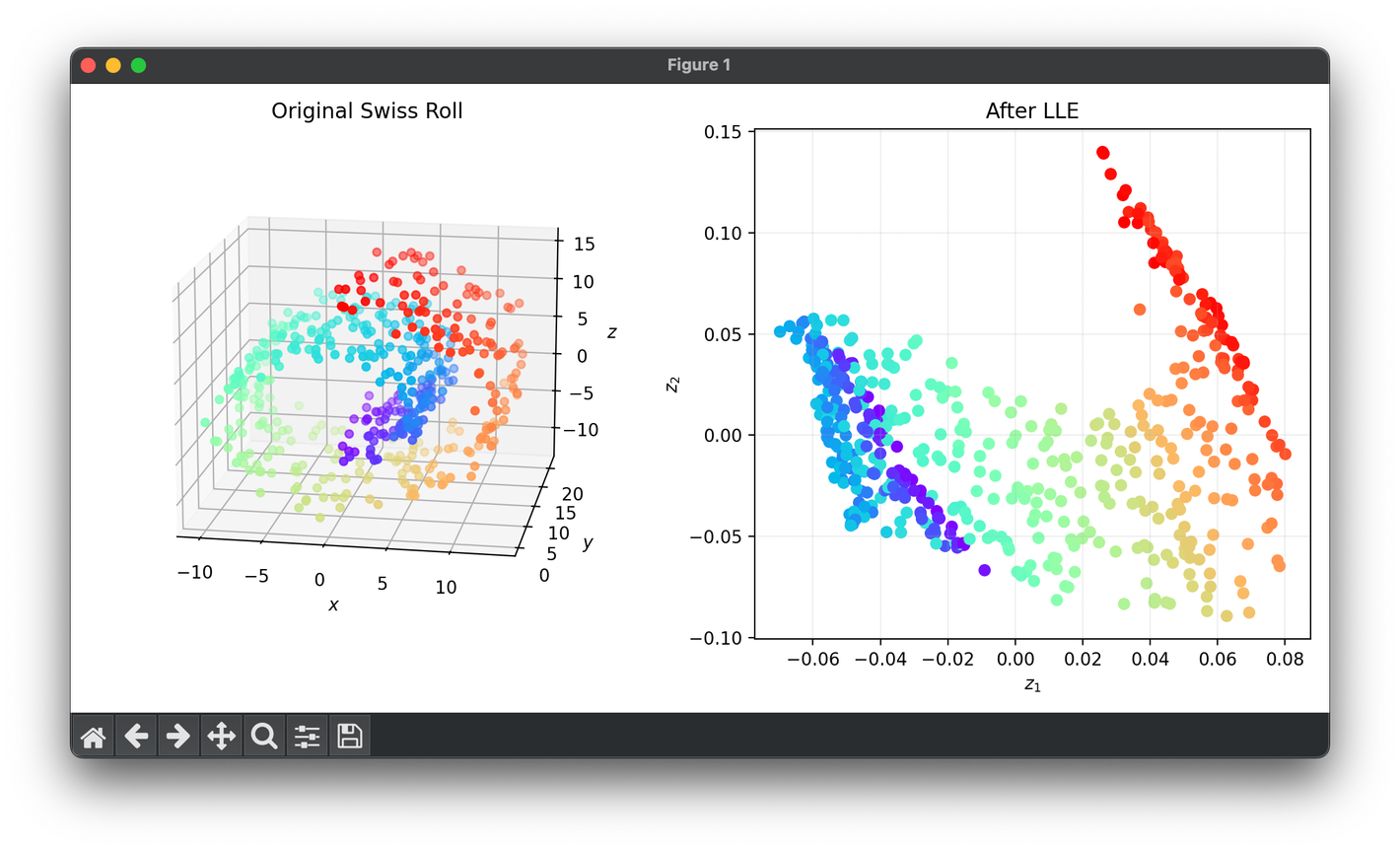
Test on the 3D Swiss-roll dataset:

from luma.reduction.manifold import LLE

from sklearn.datasets import make_swiss_roll
import matplotlib.pyplot as plt

X, y = make_swiss_roll(n_samples=500, noise=0.5)

model = LLE(n_components=2, n_neighbors=7)
Z = model.fit_transform(X)

fig = plt.figure(figsize=(10, 5))
ax1 = fig.add_subplot(1, 2, 1, projection='3d')
ax2 = fig.add_subplot(1, 2, 2)

ax1.scatter(X[:, 0], X[:, 1], X[:, 2], c=y, cmap='rainbow')
ax1.set_xlabel(r'$x$')
ax1.set_ylabel(r'$y$')
ax1.set_zlabel(r'$z$')
ax1.set_title('Original Swiss Roll')

ax2.scatter(Z[:, 0], Z[:, 1], c=y, cmap='rainbow')
ax2.set_xlabel(r'$z_1$')
ax2.set_ylabel(r'$z_2$')
ax2.set_title(f'After {type(model).__name__}')
ax2.grid(alpha=0.2)

plt.tight_layout()
plt.show()

Applications

LLE is applied in a variety of fields, including computer vision, signal processing, bioinformatics, and machine learning, particularly for tasks like data visualization, noise reduction, and feature extraction.

Strengths and Limitations

Strengths

• Non-linearity: Effective at uncovering the non-linear structure of data.
• Manifold Learning: Excels at learning the manifold structure, especially in cases where the manifold is well-defined and smooth.

Limitations

• Sensitivity to Parameters: The choice of the number of neighbors ($K$) can significantly affect the outcome.
• Data Density: Performs poorly on data with varying density.
• Optimization Challenges: Finding the global minimum of the embedding cost function can be challenging.

Advanced Topics

• Improvements and Variants: Several variants and improvements of LLE have been proposed, including modified objective functions and algorithms that better handle data with varying density or noise.
• Combination with Other Techniques: LLE can be combined with other dimensionality reduction or machine learning techniques for enhanced performance in specific tasks.

References

1. Roweis, S. T., & Saul, L. K. "Nonlinear Dimensionality Reduction by Locally Linear Embedding." Science, vol. 290, no. 5500, 2000, pp. 2323-2326.
2. Saul, L. K., & Roweis, S. T. "Think globally, fit locally: Unsupervised learning of low dimensional manifolds." Journal of Machine Learning Research, vol. 4, Jun. 2003, pp. 119-155.