Hessian Locally Linear Embedding (HLLE)

Introduction

Hessian Locally Linear Embedding (Hessian LLE) is an advanced non-linear dimensionality reduction technique used to unfold high-dimensional data into lower-dimensional spaces while preserving local geometric structures. It extends the classic Locally Linear Embedding (LLE) by incorporating second-order information through the Hessian operator, providing a more precise embedding especially in cases where the data lies on curved manifolds. This document aims to elaborate on the mathematical foundations, procedural steps, and applications of Hessian LLE, along with a discussion on its strengths and limitations.

Background and Theory

Locally Linear Embedding (LLE)

LLE starts with the assumption that each data point in a high-dimensional space can be linearly approximated by its nearest neighbors. The algorithm then seeks a low-dimensional representation of the data that preserves these local linear relationships.

Introduction to Hessian LLE

Hessian LLE enhances the LLE framework by integrating curvature information through the use of the Hessian operator. This inclusion allows for a more accurate reconstruction of the local geometry of data manifolds, making it particularly suited for data that resides on or near curved surfaces.

Mathematical Foundations

The core idea behind Hessian LLE is to use the Hessian matrix to measure the local curvature around each data point in the high-dimensional space and to preserve this curvature in the lower-dimensional embedding. This process involves several key steps:

1. Neighborhood Selection: For each data point $x_i$, select the $K$ nearest neighbors, forming a neighborhood $N_i$.

2. Weight Matrix Construction: Compute the weights $W_{ij}$ that best linearly reconstruct each data point $x_i$ from its neighbors $x_j \in N_i$, typically by minimizing the reconstruction error:

   $\epsilon(W) = \sum_i \left| x_i - \sum_{j \in N_i} W_{ij} x_j \right|^2, \quad \text{subject to} \quad \sum_{j \in N_i} W_{ij} = 1$

3. Hessian Regularization: Compute the Hessian matrix $H_i$ for each data point to measure the curvature of the local data manifold. The Hessian of a function $f$ at a point $x$ in $n$-dimensional space is given by:

   $H(f) = \left[ \frac{\partial^2 f}{\partial x_i \partial x_j} \right]_{1 \leq i,j \leq n}$

   For each neighborhood, approximate the Hessian by considering the variations in the weights $W_{ij}$ with respect to the coordinates of the data points.

4. Embedding Computation: Find a low-dimensional representation $Y$ of the data that minimizes the embedding cost function, which includes a term for preserving the local linear reconstruction weights and a regularization term based on the Hessian matrices. The optimization problem can be formulated as:

   $\Phi(Y) = \sum_i \left| y_i - \sum_{j \in N_i} W_{ij} y_j \right|^2 + \alpha \sum_i \left| H_i(Y) \right|^2$

   where $y_i$ represents the low-dimensional embedding of $x_i$, and $\alpha$ is a regularization parameter that controls the importance of the Hessian-based regularization term.

Procedural Steps

The implementation of Hessian LLE can be broken down into the following steps:

1. Data Preprocessing: Standardize the high-dimensional data to have zero mean and unit variance.
2. Neighborhood Selection: For each data point, identify the $K$ nearest neighbors.
3. Weight Matrix Construction: Solve the constrained linear least squares problem to find the weights that best reconstruct each data point from its neighbors.
4. Hessian Regularization: Approximate the Hessian matrix for each neighborhood and incorporate this second-order information into the optimization problem.
5. Embedding Optimization: Solve the optimization problem to find the low-dimensional representation that minimizes the embedding cost function, taking into account both the linear reconstruction error and the Hessian regularization term.
6. Postprocessing: Optionally, apply further normalization or scaling to the low-dimensional data.

Implementation

Parameters

• n_components: int, default = None
  Dimensionality of the lower-dimensional space
  
• n_neighbors: int, default = 5
  Number of neighbors to be considered 'close’
  
• regularization: float, default = 0.001
  Regularization parameter for stability
  

Examples

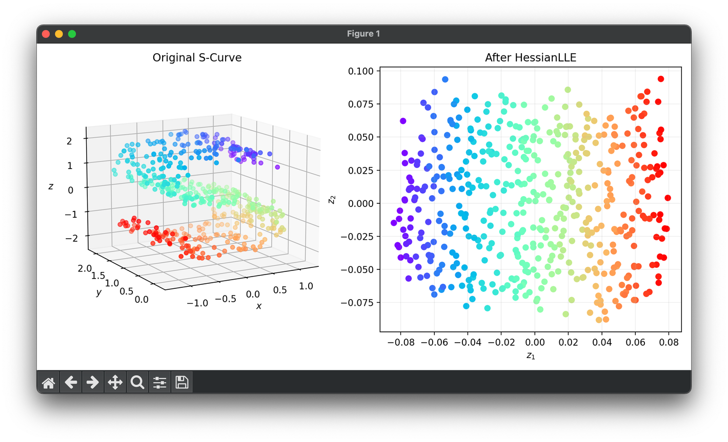
Test on the S-Curve dataset:

from luma.reduction.manifold import HessianLLE

from sklearn.datasets import make_s_curve
import matplotlib.pyplot as plt

X, y = make_s_curve(n_samples=500, noise=0.1)

model = HessianLLE(n_components=2, n_neighbors=23, regularization=1e-3)
Z = model.fit_transform(X)

fig = plt.figure(figsize=(10, 5))
ax1 = fig.add_subplot(1, 2, 1, projection='3d')
ax2 = fig.add_subplot(1, 2, 2)

ax1.scatter(X[:, 0], X[:, 1], X[:, 2], c=y, cmap='rainbow')
ax1.set_xlabel(r'$x$')
ax1.set_ylabel(r'$y$')
ax1.set_zlabel(r'$z$')
ax1.set_title('Original S-Curve')

ax2.scatter(Z[:, 0], Z[:, 1], c=y, cmap='rainbow')
ax2.set_xlabel(r'$z_1$')
ax2.set_ylabel(r'$z_2$')
ax2.set_title(f'After {type(model).__name__}')
ax2.grid(alpha=0.2)

plt.tight_layout()
plt.show()

Applications

Hessian LLE is particularly useful in applications where preserving the local and global geometric structures of high-dimensional data is critical. These include:

• Image Processing: For tasks such as image recognition and classification, where the underlying manifolds may exhibit complex curvature.
• Bioinformatics: In gene expression analysis, to uncover the intrinsic geometrical structures of high-dimensional genetic data.
• Speech Recognition: To reduce the dimensionality of feature spaces in speech signals while retaining the essential characteristics necessary for accurate recognition.

Strengths and Limitations

Strengths

• Preservation of Local Geometry: Hessian LLE's ability to incorporate curvature information makes it superior to other methods in preserving local geometric structures.
• Robustness: It is relatively robust to noise and outliers, given the incorporation of second-order information.

Limitations

• Computational Complexity: The calculation of the Hessian matrix and its regularization can be computationally intensive, especially for large datasets.
• Parameter Sensitivity: The choice of parameters, such as the number of neighbors and the regularization parameter $\alpha$, can significantly impact the quality of the embedding.

Advanced Topics

For further exploration, one might consider variations and extensions of Hessian LLE, such as adaptive neighborhood selection or integration with other manifold learning techniques to handle more complex data structures.

References

1. Donoho, David L., and Carrie Grimes. "Hessian eigenmaps: Locally linear embedding techniques for high-dimensional data." Proceedings of the National Academy of Sciences 100.10 (2003): 5591-5596.
2. Saul, Lawrence K., and Sam T. Roweis. "An Introduction to Locally Linear Embedding." 🔗
3. Roweis, Sam T., and Lawrence K. Saul. "Nonlinear dimensionality reduction by locally linear embedding." Science 290.5500 (2000): 2323-2326.