Multidimensional Scaling (MDS)

Introduction

Multidimensional Scaling (MDS) is a statistical technique used for analyzing similarity or dissimilarity data. It aims to represent data in a lower-dimensional space (typically two or three dimensions) to visualize the similarities or dissimilarities between pairs of objects. The essence of MDS is to place each object in N-dimensional space such that the between-object distances are preserved as well as possible. MDS finds its applications in various fields such as psychology, marketing, and bioinformatics, providing insightful visualizations for complex datasets.

Background and Theory

MDS is rooted in the mathematical theory of metric spaces and dimensionality reduction. The goal of MDS is to find a configuration of points in a lower-dimensional space that reflects the observed distances (similarities or dissimilarities) among a set of items as accurately as possible. The original distances are usually derived from direct measurements or computed using a distance metric such as Euclidean, Manhattan, or more complex measures that suit the data characteristics.

Mathematical Foundations

Given a set of $n$ items with a matrix $\mathbf{D}$ representing the dissimilarities between each pair of items, MDS seeks a set of $n$ points in $p$ dimensions (where $p < n$), such that the Euclidean distances between these points closely match the original dissimilarities. The objective is to minimize the stress function $S$, which is a measure of the discrepancy between the distances in the lower-dimensional representation and the original dissimilarities:

where $d_{ij}$ is the Euclidean distance between points $i$ and $j$ in the lower-dimensional space, and $\delta_{ij}$ is the original dissimilarity between items $i$ and $j$.

Types of MDS

• Classical MDS: Assumes the dissimilarity measures are Euclidean and works best when the original distances can be accurately represented in the lower-dimensional space.
• Nonmetric MDS: Relaxes the assumption of Euclidean distances and focuses on preserving the rank order of the dissimilarities rather than their exact values.

Procedural Steps

1. Input Data: Begin with a matrix of observed dissimilarities $\mathbf{D}$.
2. Distance Matrix Computation: If $\mathbf{D}$ is not a distance matrix, convert the similarities to distances or normalize the dissimilarities as required.
3. Configuration Initialization: Initialize a configuration of $n$ points in a $p$-dimensional space. This can be done randomly or based on some heuristic.
4. Stress Minimization: Use an optimization technique (such as gradient descent or majorization) to adjust the positions of the points in order to minimize the stress function $S$.
5. Iteration: Repeat the optimization process until $S$ converges to a minimum value or until a predetermined number of iterations is reached.
6. Output: The final configuration of points represents the items in a lower-dimensional space, reflecting their similarities or dissimilarities.

Implementation

Parameters

• n_components: int, default = None
  Dimensionality of low-space
  

Examples

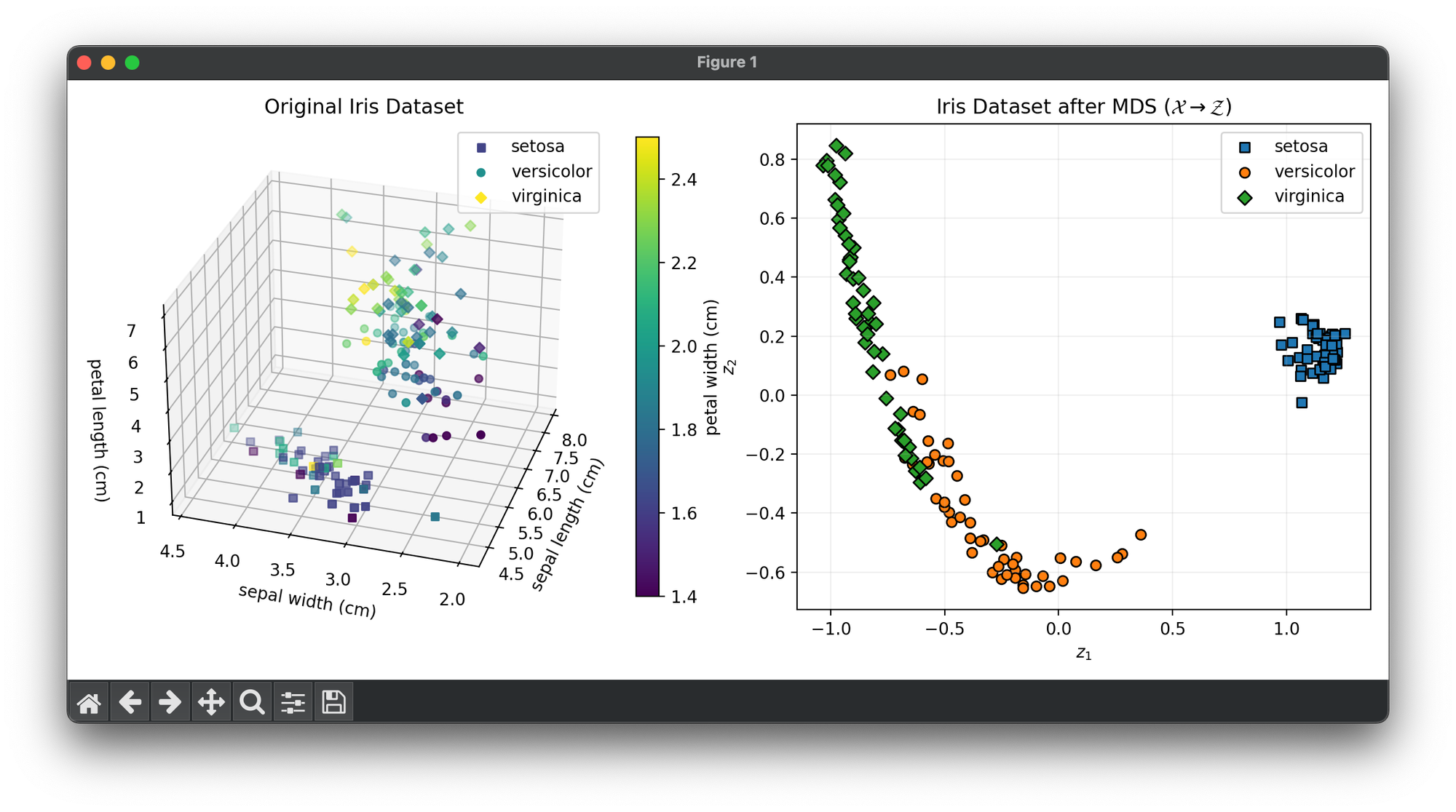
Test on the wine dataset:

from luma.reduction.manifold import MDS

from sklearn.datasets import load_iris

import matplotlib.pyplot as plt
import numpy as np

iris_df = load_iris()
X = iris_df.data
y = iris_df.target

model = MDS(n_components=2)
X_trans = model.fit_transform(X)

fig = plt.figure(figsize=(11, 5))
ax1 = fig.add_subplot(1, 2, 1, projection="3d")
ax2 = fig.add_subplot(1, 2, 2)

for cl, m in zip(np.unique(y), ["s", "o", "D"]):
    X_cl = X[y == cl]
    sc = ax1.scatter(
        X_cl[:, 0],
        X_cl[:, 1],
        X_cl[:, 2],
        c=X_cl[:, 3],
        marker=m,
        label=iris_df.target_names[cl],
    )

ax1.set_xlabel(iris_df.feature_names[0])
ax1.set_ylabel(iris_df.feature_names[1])
ax1.set_zlabel(iris_df.feature_names[2])
ax1.set_title("Original Iris Dataset")
ax1.legend()

cbar = ax1.figure.colorbar(sc, fraction=0.04)
cbar.set_label(iris_df.feature_names[3])

for cl, m in zip(np.unique(y), ["s", "o", "D"]):
    X_tr_cl = X_trans[y == cl]
    ax2.scatter(
        X_tr_cl[:, 0],
        X_tr_cl[:, 1],
        marker=m,
        edgecolors="black",
        label=iris_df.target_names[cl],
    )

ax2.set_xlabel(r"$z_1$")
ax2.set_ylabel(r"$z_2$")
ax2.set_title(
    f"Iris Dataset after {type(model).__name__} "
    + r"$(\mathcal{X}\rightarrow\mathcal{Z})$"
)
ax2.legend()
ax2.grid(alpha=0.2)

plt.tight_layout()
plt.show()

Applications

MDS is versatile and finds applications across various domains:

• Market Research: To visualize consumer preferences and segment markets based on product similarity perceptions.
• Bioinformatics: For genetic and protein structure analysis, where similarities/dissimilarities are based on sequence or functional similarities.
• Psychometrics: To understand the dimensions underlying psychological measures or tests.
• Information Visualization: For visualizing the structure of information spaces, like similarities among documents or websites.

Strengths and Limitations

Strengths

• Flexibility: Can handle a wide variety of dissimilarity measures.
• Intuitive Visualizations: Provides a straightforward way to visualize complex relationships in data.
• Applicability: Useful in fields where the data is inherently multidimensional and complex.

Limitations

• Dimensionality: Choosing the number of dimensions ($p$) can be challenging and may affect the interpretation.
• Stress Function Sensitivity: The outcome is sensitive to the choice of stress function and optimization technique.
• Interpretability: The dimensions in the lower-dimensional space may not always have a clear interpretation.

Advanced Topics

• Metric Selection: The choice of distance metric can significantly affect the MDS outcomes. Exploring different metrics based on data characteristics is crucial.
• MDS Algorithms: Various algorithms offer different approaches to minimizing the stress function, each with its own advantages.
• Hybrid Techniques: Combining MDS with other dimensionality reduction techniques (like PCA or t-SNE) can provide complementary insights.

References

1. Borg, I., & Groenen, P. J. (2005). Modern Multidimensional Scaling: Theory and Applications. Springer Series in Statistics. Springer.
2. Cox, T. F., & Cox, M. A. (2001). Multidimensional Scaling. Chapman and Hall/CRC.
3. Kruskal, J. B., & Wish, M. (1978). Multidimensional Scaling. Sage Publications.