Ridge Regression

Introduction

Ridge regression, also known as Tikhonov regularization, is a technique used for analyzing multiple regression data that suffer from multicollinearity. By adding a degree of bias to the regression estimates, ridge regression reduces the standard errors. It's particularly useful when the predictor variables are highly correlated or when the number of predictors exceeds the number of observations.

This document delves into the mathematical optimization process underlying ridge regression, detailing its theoretical foundation, procedural steps, and mathematical formulations. It aims to provide a comprehensive understanding of the algorithm, its applications, strengths, limitations, and relevant advanced topics.

Background and Theory

Linear Regression Recap

Linear regression models the relationship between a dependent variable $Y$ and one or more independent variables denoted as $X$. The model is given by:

where $\beta_0, \beta_1, \cdots, \beta_p$ are coefficients, and $\epsilon$ represents the error term.

The Issue of Multicollinearity

Multicollinearity occurs when independent variables in a regression model are highly correlated. This can lead to inflated standard errors and unreliable coefficient estimates.

Ridge Regression

Ridge regression addresses multicollinearity by adding a penalty (the ridge penalty) to the size of coefficients. This penalty is a function of the sum of the squares of the coefficients, leading to the optimization problem:

where $\lambda \geq 0$ is the tuning parameter that controls the strength of the penalty.

Mathematical Formulation

Objective Function

The objective in ridge regression is to minimize the penalized residual sum of squares (RSS):

where $L(\beta)$ is the loss function, $\|\boldsymbol{\beta}\|^2_2$ denotes the squared Euclidean norm (L2 norm) of the coefficient vector $\boldsymbol{\beta}$, excluding $\beta_0$.

Optimization Process

1. Gradient Descent: To find the coefficients that minimize $L(\beta)$, one approach is gradient descent, where coefficients are iteratively updated in the direction that most steeply decreases the loss function.

2. Analytical Solution: The ridge regression coefficients can also be found analytically by setting the gradient of $L(\beta)$ with respect to $\beta$ to zero:

   $\frac{\partial L(\beta)}{\partial \beta} = -2X^T(Y - X\beta) + 2\lambda\beta = 0$

   Solving for $\beta$ gives:

   $\beta = (X^TX + \lambda I)^{-1}X^TY$

   where $I$ is the identity matrix of size $(p+1) \times (p+1)$ (assuming the first element is associated with $\beta_0$ and $\lambda$ is not applied to it).

Implementation

Parameters

• alpha: float, default = 1.0
  L2 regularization strength
  

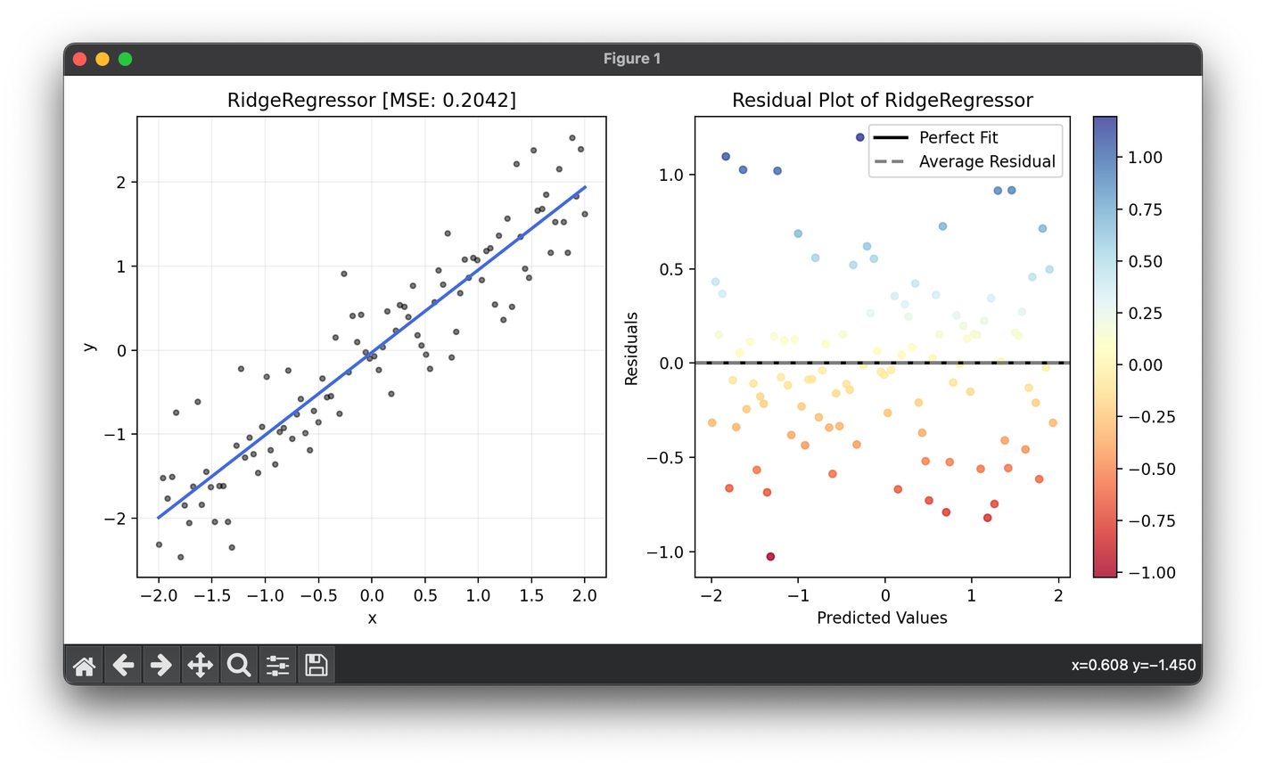
Examples

from luma.regressor.linear import RidgeRegressor
from luma.model_selection.search import GridSearchCV
from luma.metric.regression import MeanSquaredError
from luma.visual.evaluation import ResidualPlot

import matplotlib.pyplot as plt
import numpy as np

X = np.linspace(-2, 2, 100).reshape(-1, 1)
y = X.flatten() + 0.5 * np.random.randn(100)

param_grid = {"alpha": np.logspace(-3, 3, 10)}

grid = GridSearchCV(estimator=RidgeRegressor(),
                    param_grid=param_grid,
                    cv=5,
                    metric=MeanSquaredError,
                    maximize=False,
                    refit=True,
                    shuffle=True,
                    random_state=42)

grid.fit(X, y)
print(grid.best_params, grid.best_score)
reg = grid.best_model

fig = plt.figure(figsize=(10, 5))
ax1 = fig.add_subplot(1, 2, 1)
ax2 = fig.add_subplot(1, 2, 2)

ax1.scatter(X, y, s=10, c="black", alpha=0.5, label=r"y=x+\epsilon")
ax1.plot(X, reg.predict(X), lw=2, c="royalblue")
ax1.set_xlabel("x")
ax1.set_ylabel("y")
ax1.set_title(f"{type(reg).__name__} [MSE: {reg.score(X, y):.4f}]")
ax1.grid(alpha=0.2)

res = ResidualPlot(reg, X, y)
res.plot(ax=ax2, show=True)

Applications

Ridge regression is widely used in situations where linear regression would likely overfit or when the data is multicollinear. Some common applications include:

• Finance: For predicting stock prices based on various economic factors.
• Healthcare: In genomic data analysis where the number of predictors (genes) far exceeds the number of observations (patients).
• Marketing: To predict consumer behavior based on historical data involving a large number of predictor variables.

Strengths and Limitations

Strengths

• Reduces Overfitting: By introducing a penalty term, ridge regression reduces the complexity of the model, which can help in preventing overfitting.
• Handles Multicollinearity: It provides a way to deal with multicollinearity by shrinking the coefficients of correlated predictors.

Limitations

• Selection of $\lambda$: Choosing the right value for $\lambda$ is critical and can be challenging. Cross-validation techniques are typically employed to select an optimal $\lambda$.
• Bias: The model introduces bias into the estimates for the sake of reducing variance.

Advanced Topics

Kernel Ridge Regression

Kernel ridge regression extends ridge regression to nonlinear models by employing kernel functions. This allows the algorithm to fit nonlinear relationships without explicitly transforming the input features into a high-dimensional space.

Cross-Validation for $\lambda$ Selection

Cross-validation techniques, such as k-fold cross-validation, are essential for choosing an appropriate $\lambda$. The goal is to find a $\lambda$ that minimizes the cross-validation error, balancing bias and variance.

References

1. Hoerl, Arthur E., and Robert W. Kennard. "Ridge regression: Biased estimation for nonorthogonal problems." Technometrics 12.1 (1970): 55-67.
2. Tikhonov, Andrey N. "Solution of incorrectly formulated problems and the regularization method." Soviet Math. Dokl. 4 (1963): 1035-1038.
3. Hastie, Trevor, Robert Tibshirani, and Jerome Friedman. The Elements of Statistical Learning. Springer Series in Statistics. Springer New York Inc., 2001.