Lasso Regression

Introduction

Lasso regression, standing for Least Absolute Shrinkage and Selection Operator, is a regression analysis method that performs both variable selection and regularization in order to enhance the prediction accuracy and interpretability of the statistical model it produces. Unlike ridge regression, which only shrinks coefficients, lasso has the ability to set coefficients to zero, effectively selecting a simpler model that does not include those variables.

This document provides a comprehensive exploration of lasso regression, focusing on its theory, mathematical formulations, procedural steps, applications, strengths, limitations, and advanced topics related to the algorithm.

Background and Theory

Overview of Linear Regression

Linear regression aims to model the relationship between a dependent variable $Y$ and one or more independent variables $X$. The model is:

Here, $\beta_0, \beta_1, \cdots, \beta_p$ are the coefficients, and $\epsilon$ is the error term.

The Lasso Approach

Lasso regression modifies the loss function to include a penalty on the absolute size of the coefficients. This penalty term leads to some coefficients being exactly zero when the penalty is sufficiently large, which means lasso performs variable selection.

The lasso optimization problem is formulated as:

where $\lambda \geq 0$ is the regularization parameter that controls the amount of shrinkage applied to the coefficients.

Mathematical Formulation

Objective Function

The objective in lasso regression is to minimize the penalized residual sum of squares (RSS):

where $\|\boldsymbol{\beta}\|_1$ denotes the L1 norm of the coefficient vector $\boldsymbol{\beta}$, emphasizing that lasso penalty involves the sum of the absolute values of the coefficients.

Solving the Optimization Problem

The lasso problem does not have a closed-form solution like ridge regression because the L1 penalty makes the optimization problem non-differentiable at zero. Instead, numerical methods such as coordinate descent or the least angle regression (LARS) algorithm are commonly used to find the coefficients.

Implementation

Parameters

• alpha: float, default = 1.0
  L1 regularization strength
  
• learning_rate: float, default = 0.01
  Step size of the gradient descent update
  
• max_iter: int, default = 100
  Number of iteration
  

Examples

from luma.regressor.linear import LassoRegressor
from luma.model_selection.search import GridSearchCV
from luma.metric.regression import MeanSquaredError
from luma.visual.evaluation import ResidualPlot

import matplotlib.pyplot as plt
import numpy as np

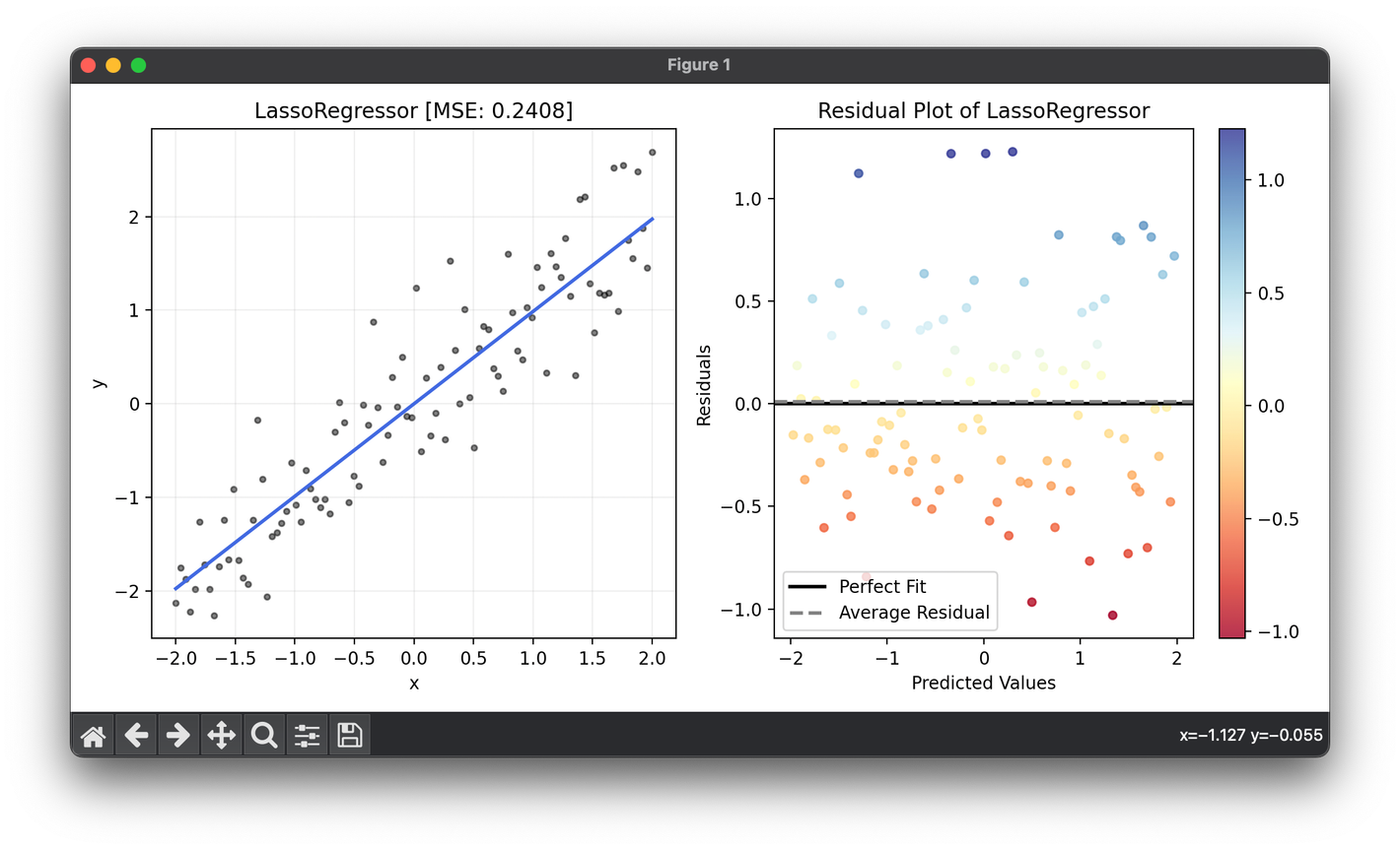
X = np.linspace(-2, 2, 100).reshape(-1, 1)
y = X.flatten() + 0.5 * np.random.randn(100)

param_grid = {"alpha": np.logspace(-3, 3, 5),
              "learning_rate": np.logspace(-3, -1, 5)}

grid = GridSearchCV(estimator=LassoRegressor(),
                    param_grid=param_grid,
                    cv=5,
                    metric=MeanSquaredError,
                    maximize=False,
                    refit=True,
                    shuffle=True,
                    random_state=42)

grid.fit(X, y)
print(grid.best_params, grid.best_score)
reg = grid.best_model

fig = plt.figure(figsize=(10, 5))
ax1 = fig.add_subplot(1, 2, 1)
ax2 = fig.add_subplot(1, 2, 2)

ax1.scatter(X, y, s=10, c="black", alpha=0.5, label=r"y=x+\epsilon")
ax1.plot(X, reg.predict(X), lw=2, c="royalblue")
ax1.set_xlabel("x")
ax1.set_ylabel("y")
ax1.set_title(f"{type(reg).__name__} [MSE: {reg.score(X, y):.4f}]")
ax1.grid(alpha=0.2)

res = ResidualPlot(reg, X, y)
res.plot(ax=ax2, show=True)

Applications

Lasso regression is widely used in fields where model interpretability is crucial, such as in:

• Bioinformatics: For genetic data where the number of predictors (genes) far exceeds the number of observations.
• Finance: In risk management and predictive modeling of financial assets.
• Environmental Science: For climate modeling and forecasting where selecting the most significant variables is crucial.

Strengths and Limitations

Strengths

• Variable Selection: Lasso's ability to reduce some coefficients to zero can simplify models and highlight significant variables.
• Predictive Accuracy: By eliminating irrelevant variables, lasso can improve the model's predictive accuracy, especially in cases of high-dimensional data.

Limitations

• Selection of $\lambda$: Choosing the correct value for $\lambda$ is critical and can significantly affect model performance. Cross-validation is typically used to select an optimal $\lambda$.
• Bias: For very high values of $\lambda$, lasso can introduce significant bias into the model, trading off variance for bias.

Advanced Topics

Elastic Net

Elastic Net is an extension of lasso that combines the penalties of ridge regression and lasso, benefiting from both their properties. It is particularly useful when there are multiple features correlated with each other.

Adaptive Lasso

Adaptive lasso varies the penalty level for different coefficients, allowing for more flexibility in variable selection. It aims to overcome some of the limitations of the standard lasso method, particularly in terms of variable selection consistency.

References

1. Tibshirani, Robert. "Regression shrinkage and selection via the lasso." Journal of the Royal Statistical Society: Series B (Methodological) 58.1 (1996): 267-288.
2. Zou, Hui, and Trevor Hastie. "Regularization and variable selection via the elastic net." Journal of the Royal Statistical Society: Series B (Statistical Methodology) 67.2 (2005): 301-320.
3. Zou, Hui. "The adaptive lasso and its oracle properties." Journal of the American Statistical Association 101.476 (2006): 1418-1429.