Logistic Regression
논리 회귀(Logistic Regression)는 데이터를 그룹화해서 특정 라벨로 분류하는 분석 방법이다. 주어진 입력값에 어떤 라벨이 적합한지 반환한다. 마치 우리가 빨갛고 둥그런 과일을 사과라고 판단하는 것과 유사하다. 즉, 미리 학습된 Logistic Regression 모델에 (빨간색, 구, 과일)의 입력값을 주면, 이에 대해 사과라는 값을 반환하는 일종의 함수다.
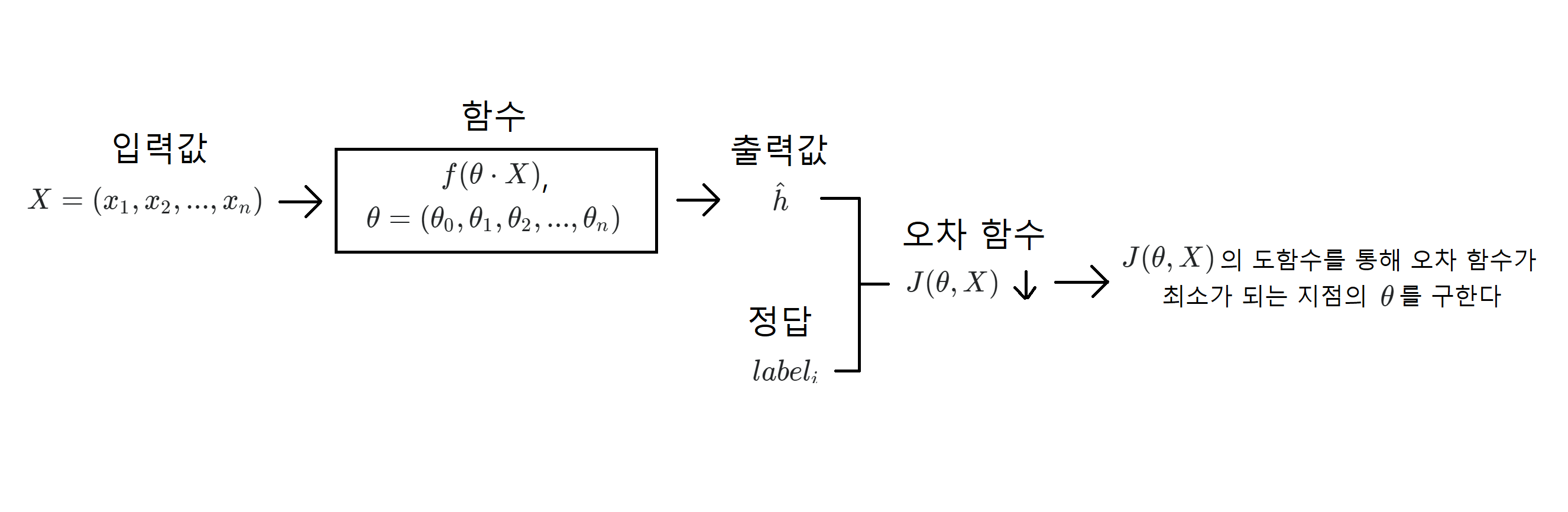
일반적으로 기계 학습 중 지도 학습은 입력값과 정답이 주어지고, 거기에 대해 적절한 분류 함수와 그에 따른 오차 함수를 설계하여 오차를 최소화하는 를 구한다. 이 를 구하는 과정을 학습이라고 표현한다. 그리고 위 그림에서 함수(모델 함수)가 데이터 분류에 실제로 사용되는 함수다.
기계 학습은 모델 함수와 오차 함수를 적절하게 설계하는 것이 중요하다. 모델 함수는 여러 종류가 있으며 각각의 장단점이 존재하기 때문에 장단점을 고려해 학습 목적에 적합한 함수를 사용하고, 오차 함수는 도함수를 구해야하기 때문에 미분이 수월하도록 설계한다.
1. 데이터 표현하기
# 1. Plot the training data [2pt]

import numpy as np
import matplotlib.pyplot as plt

# load the training data file ('data.txt')
data = np.genfromtxt("drive/My Drive/.../data.txt", delimiter=',')

# each row (xi,yi,li) of the data consists of a 2-dimensional point (x,y) with its label l
# x,y ∈ R
x = data[:, 0]
y = data[:, 1]
# l ∈ {0,1}
label = np.array(list(map(int, data[:, 2])))

# get x by label
x_label0 = x[label == 0]
x_label1 = x[label == 1]

# get y by label
y_label0 = y[label == 0]
y_label1 = y[label == 1]

# plot the training data points (x,y) with their labels l
plt.figure(figsize=(8, 8))
# in colors (blue for label 0 and red for label 1)
plt.scatter(x_label0, y_label0, color='blue')
plt.scatter(x_label1, y_label1, color='red')
plt.show()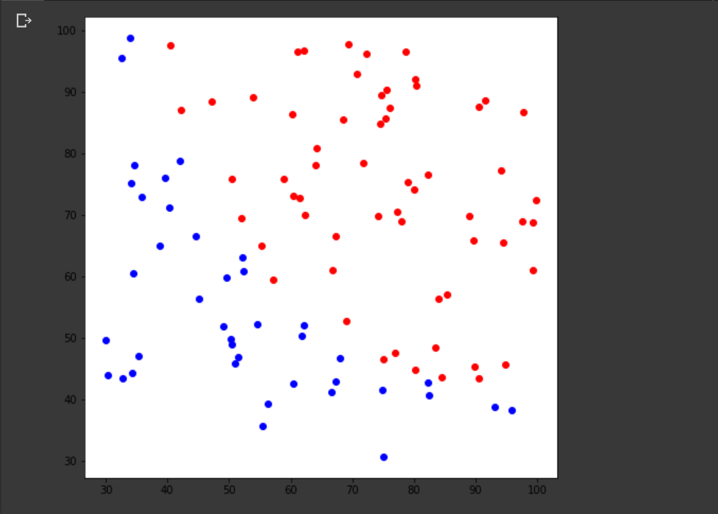
data.txt 파일은 각 행마다 값이 저장되어 있다. 는 실수에 속하고 은 0 또는 1의 정수이다. 그리고 라벨이 0이면 파란색으로 라벨이 1이면 빨간색으로 설정해 화면에 표시했다.
2. 모델 파라미터 변화량 표현하기
# 2. Plot the estimated parameters [3pt]
import numpy as np
import matplotlib.pyplot as plt
from math import *
from decimal import Decimal
# Logistic regression
def h(z):
return 1 / (1 + np.exp(-z))
# Gradient Descent
def get_next_theta(theta, j, data, learning_rate):
sumation = 0
for i in data:
X = np.array([1, i[0], i[1]])
z = theta @ X
sumation += (h(z) - i[2]) * X[j]
return theta[j] - learning_rate * (1 / len(data)) * sumation
def is_converged(theta, next_theta):
for i in range(len(theta)):
if(Decimal(theta[0]) != Decimal(next_theta[0])):
return False
return True
# load the training data file ('data.txt')
data = np.genfromtxt("drive/My Drive/.../data.txt", delimiter=',')
# you can use any initial conditions (θ0,θ1,θ2)
theta = np.array([-10, 0, 10], 'float64')
# you should choose a learning rate α in such a way that the convergence is achieved
learning_rate = 0.001
# the estimated parameters (θ0,θ1,θ2) at every iteration of gradient descent
theta0 = [theta[0]]
theta1 = [theta[1]]
theta2 = [theta[2]]
# find optimal parameters (θ0,θ1,θ2) using the training data
while True:
next_theta = np.empty(3, 'float64')
next_theta[0] = get_next_theta(theta, 0, data, 100 * learning_rate)
next_theta[1] = get_next_theta(theta, 1, data, learning_rate)
next_theta[2] = get_next_theta(theta, 2, data, learning_rate)
# break the loop if all parameters are converged
if(is_converged(theta, next_theta)):
break
# save the theta
theta0.append(next_theta[0])
theta1.append(next_theta[1])
theta2.append(next_theta[2])
# update the theta
theta = next_theta
print(len(theta0))
print('Theta:', theta)
# plot the estimated parameters (θ0,θ1,θ2) at every iteration of gradient descent until convergence
plt.figure(figsize=(8, 8))
# the colors for the parameters (θ0,θ1,θ2) should be red, green, blue, respectively
x = range(len(theta0))
plt.plot(x, theta0, color='red')
plt.plot(x, theta1, color='green')
plt.plot(x, theta2, color='blue')
plt.show()
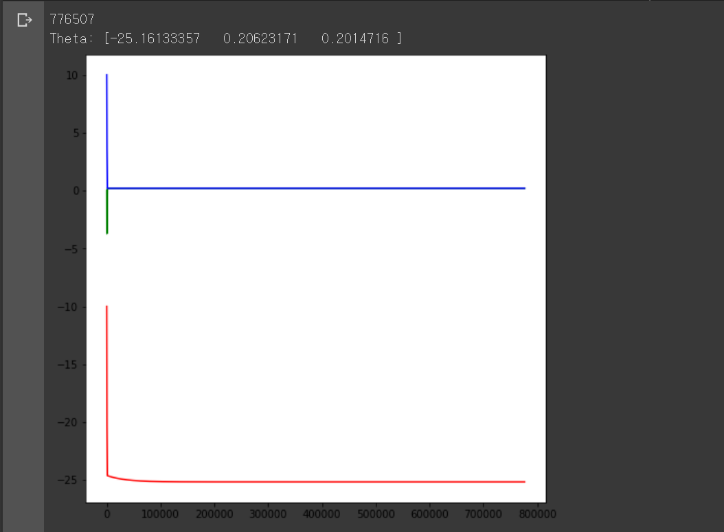
모델 파라미터
우리가 원하는 것은 어떠한 입력을 줬을 때 특정 라벨을 반환하는 모델을 만드는 것이다. 일반적으로 입력값은 여러 개의 수로 이뤄져 있고 출력값은 1개이기 때문에 입력값을 1개의 수로 변환하는 작업을 거친다. 여기서 는 입력값이고 는 모델 파라미터다.
이를 n개의 요소에 대해 일반화하면 다음과 같다.
,
,
, where
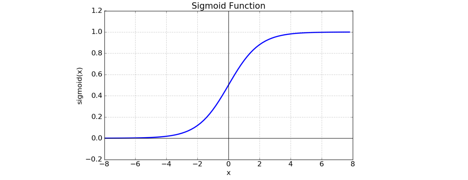
이제 이 값을 특정 함수에 넣었을 때의 출력값으로 분류를 할 것이다. 여기엔 여러 종류의 함수가 사용될 수 있는데 이번에는 sigmoid 함수를 사용할 것이다. Sigmoid 함수의 특성은 아래와 같다.
Sigmoid 함수
-
-
-
점 을 지난다.
-
이고, 이다.
-
도함수는 이다.
위 학습 데이터는 라벨이 0 또는 1로 2가지 존재하기 때문에 가 1에 가까우면 라벨을 1로 분류하고 0에 가까우면 0으로 분류한다.
오차 함수
경사하강법
이제 우리는 학습데이터에 경사하강법을 적용해 적절한 를 구하려고 한다. 경사하강법을 적용한 는 다음과 같다.
-
,
-
,
-
,
여기서 뒤에 곱해진 부분은 각각의 로 미분한 오차 함수의 도함수이다.
3. 손실 함수 변화량 표현하기
# 3. Plot the training error [3pt]

import numpy as np
import matplotlib.pyplot as plt
from math import *
from decimal import Decimal


# Logistic regression
def h(z):
  z = 0.001 * z
  return 1 / (1 + np.exp(-z))

# Objective Function
def J(theta, data):
  sumation = 0
  for i in data:
    z = theta @ np.array([1, i[0], i[1]])
    sumation += -i[2] * log(h(z)) - (1 - i[2]) * log(1 - h(z))
  return (1 / len(data)) * sumation

# Gradient Descent
def get_next_theta(theta, j, data, learning_rate):
  sumation = 0
  for i in data:
    X = np.array([1, i[0], i[1]])
    z = theta @ X
    sumation += (h(z) - i[2]) * X[j]
  return theta[j] - learning_rate * (1 / (1000 * len(data))) * sumation

def is_converged(theta, next_theta):
  for i in range(len(theta)):
    if(Decimal(theta[0]) != Decimal(next_theta[0])):
      return False
  return True


# load the training data file ('data.txt')
data = np.genfromtxt("drive/My Drive/.../data.txt", delimiter=',')

# you can use any initial conditions (θ0,θ1,θ2)
theta = np.array([-2000, -1000, 0], 'float64')

# you should choose a learning rate α in such a way that the convergence is achieved
learning_rate = 1000

# the training error J(θ0,θ1,θ2) at every iteration of gradient descent until convergence
J_theta = [J(theta, data)]

# find optimal parameters (θ0,θ1,θ2) using the training data
while True:
  next_theta = np.empty(3, 'float64')
  next_theta[0] = get_next_theta(theta, 0, data, 100 * learning_rate)
  next_theta[1] = get_next_theta(theta, 1, data, learning_rate)
  next_theta[2] = get_next_theta(theta, 2, data, learning_rate)

  # break the loop if parameters are converged
  if(is_converged(theta, next_theta)):
    break

  # save the training error J(θ0,θ1,θ2)
  J_theta.append(J(next_theta, data))

  # update the theta
  theta = next_theta

print(len(J_theta))
print('Theta:', theta)

# plot the estimated parameters (θ0,θ1,θ2) at every iteration of gradient descent until convergence
plt.figure(figsize=(8, 8))

# the colors for the training error J(θ0,θ1,θ2) should be blue
plt.plot(range(len(J_theta)), J_theta, color='blue')
plt.show()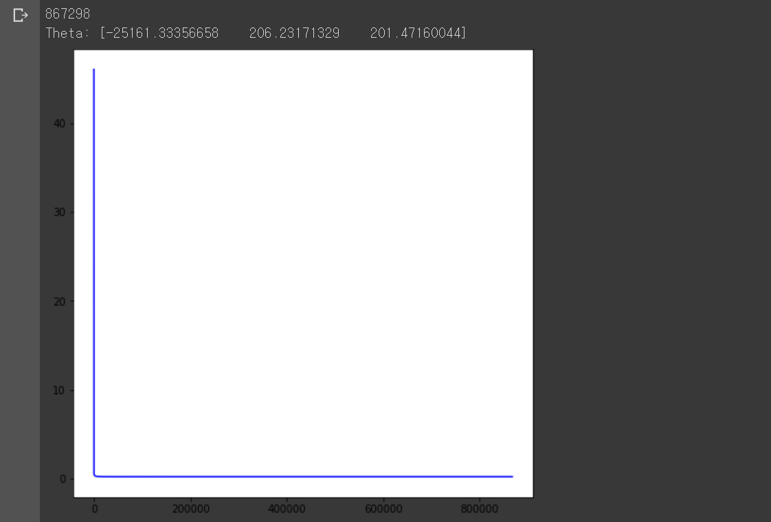
이번에는 경사하강법 각 단계별 오차 함숫값이 어떻게 변하는지 표현했다. 도함수를 통해 오차 함수가 감소하는 방향으로 를 변화시켰기 때문에 함숫값이 점점 감소하는 그래프가 그려졌다. 축이 길어서 함숫값이 감소하는 모습이 잘 보이지 않지만 확대해서 보면 점점 감소하는 모습으로 그려졌다.
2번과 비교해서 코드는 경사하강법 매 단계마다 값 대신 오차 함수 값을 저장하고, 저장한 값을 그래프로 그린 것 이외에는 달라진 점이 없다.
4. 학습된 모델 표현하기
# 4. Plot the obtained classifier [4pt]

import numpy as np
from matplotlib import pyplot as plt
from matplotlib import cm
from math import *
from decimal import Decimal


# Logistic regression
def h(z):
  z = 0.001 * z
  return 1 / (1 + np.exp(-z))

# Objective Function
def J(theta, data):
  sumation = 0
  for i in data:
    z = theta @ np.array([1, i[0], i[1]])
    sumation += -i[2] * log(h(z)) - (1 - i[2]) * log(1 - h(z))
  return (1 / len(data)) * sumation

# Gradient Descent
def get_next_theta(theta, j, data, learning_rate):
  sumation = 0
  for i in data:
    X = np.array([1, i[0], i[1]])
    z = theta @ X
    sumation += (h(z) - i[2]) * X[j]
  return theta[j] - learning_rate * (1 / (1000 * len(data))) * sumation

def is_converged(theta, next_theta):
  for i in range(len(theta)):
    if(Decimal(theta[0]) != Decimal(next_theta[0])):
      return False
  return True


# load the training data file ('data.txt')
data = np.genfromtxt("drive/My Drive/.../data.txt", delimiter=',')

# each row {(x_i, y_i, l_i)} of the data consists of a 2-dimensional point (x,y) with its label l
# x,y ∈ R and l ∈ {0,1}
x = data[:, 0]
y = data[:, 1]
label = data[:, 2]

x_label0 = x[label == 0]
x_label1 = x[label == 1]

y_label0 = y[label == 0]
y_label1 = y[label == 1]

# you can use any initial conditions (θ0,θ1,θ2)
theta = np.array([-2000, -1000, 0], 'float64')

# you should choose a learning rate α in such a way that the convergence is achieved
learning_rate = 1000

# the step count of gradient descent
count = 0

# find optimal parameters (θ0,θ1,θ2) using the training data
while True:
  next_theta = np.empty(3, 'float64')
  next_theta[0] = get_next_theta(theta, 0, data, 100 * learning_rate)
  next_theta[1] = get_next_theta(theta, 1, data, learning_rate)
  next_theta[2] = get_next_theta(theta, 2, data, learning_rate)

  # break the loop if parameters are converged
  if(is_converged(theta, next_theta)):
    break

  # save the training error J(θ0,θ1,θ2)
  J_theta.append(J(next_theta, data))

  # update the theta and count of gradient descent
  theta = next_theta
  count += 1

print(count)
print('Theta:', theta)

# the classifier σ(z) where z=θ0+θ1x+θ2y with x=[30:0.5:100] and y=[30:0.5:100]
X = np.arange(30, 100, 0.5)
Y = np.arange(30, 100, 0.5)
X, Y = np.meshgrid(X, Y)
Z = theta[0] + theta[1] * X + theta[2] * Y

# plot the estimated parameters (θ0,θ1,θ2) at every iteration of gradient descent until convergence
plt.figure(figsize=(8, 8))
plt.imshow(h(Z), cmap=cm.coolwarm, vmin=0, vmax=1)

# [a:t:b] denotes a range of values from a to b with a stepsize t
ax = plt.gca()
ax.invert_yaxis()
ax.set_xlim(30, 100)
ax.set_ylim(30, 100)

# in colors (blue for label 0 and red for label 1)
plt.scatter(x_label0, y_label0, color='blue')
plt.scatter(x_label1, y_label1, color='red')
plt.show()
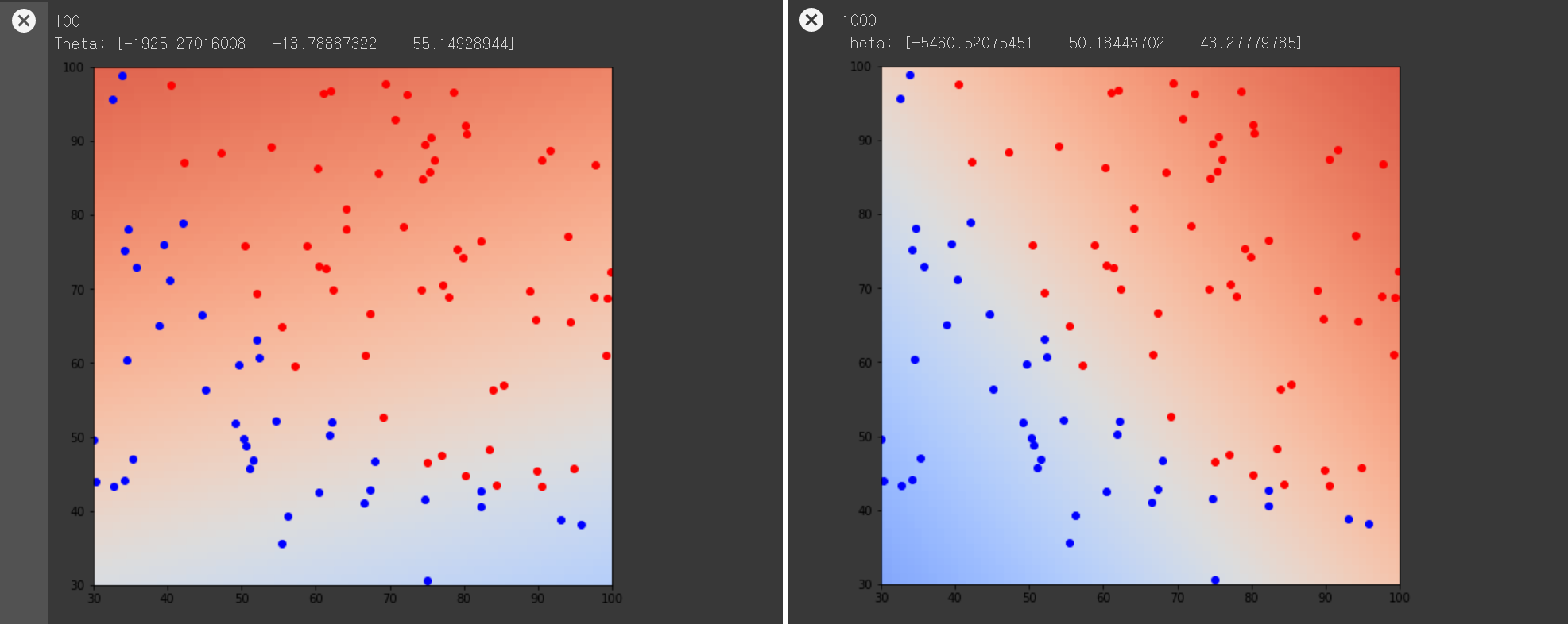

1번에서 파란색 점을 라벨 0으로, 빨간색 점을 라벨 1로 표현한 그림 위에 학습한 시그모이드 모델을 표현한 그림이다. 위와 같이 경사하강법 단계를 거듭할수록 색의 구분이 명확해지고 색상이 진해지는 것을 볼 수 있다.

2개의 댓글

With Beautykhan’s Escort in Gurgaon you will embrace sophistication and encounter gorgeous and intelligent companions who will be a delight to engage with. One of our top priorities is to ensure complete confidentiality so that our clients can enjoy our services in as much comfort as possible, knowing that we respect their right to privacy.
Have you seen any 'hindu muslim sex story hindi' content? The language and cultural context make these stories stand out. It's a fresh and exciting read.