딥러닝

머신러닝과 비교

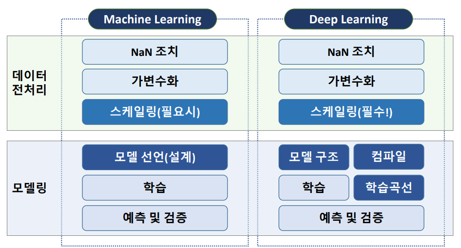
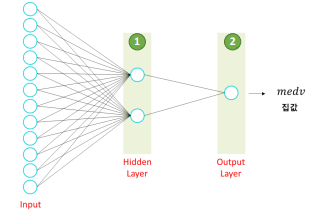
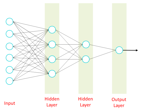
딥러닝 구조

layer

• 입력층(Input), 은닉층(Hidden), 출력층(Output) 으로 구성
  

# Sequential 타입 모델 선언(입력은 리스트로!)
model3 = Sequential([Input(shape = (nfeatures,)),
				  ① Dense(2, activation = 'relu'), #hidden layer
				  ② Dense(1) ])

• layer 여러개 : 리스트로 입력
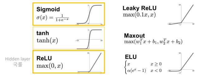
• ① hidden layer : Activation : 활성함수는 보통 'relu'사용
• ② output layer : 예측 결과가 1개

💡활성화 함수 : 현재 레이어(각노드)의 결과값을 다음 레이어로 어떻게 전달할지 결정/변환해주는 함수
없으면 hidden layer를 아무리 추가해도 선형회귀임

hidden layer : 선형을 비선형 함수로 변환
output layer : 결과값을 다른 값으로 변환 (주로 분류모델)

process

• 각 단계 task는 input을 처리 후 전달

Input > task1 ... taskn > Output

Dense

• Input : Input(shape = ( , ))
  • 분석단위에 대한 shape
    • 1차원 : (feature 수, )
    • 2차원 : (rows, columns)
• OutPut : Dense( )
  • 예측결과 1개 변수

Compile

model.compile(optimizer = Adam(learning_rate = 0.1), loss='mse')

• loss (오차함수)
  • 오차계산을 뭐로 할지 결정
  • 회귀 : mse, 분류 : cross entropy

optimizer

• 오차를 최소화하도록 가중치를 업데이트 하는 역할
• Adam : 최근 딥러닝에서 가장 성능이 좋은 opmz로 평가
• learning_rate : 학습율, 기울기에 곱해지는 조정비율 (보폭)

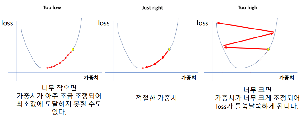
learning_rate

• 가중치
  

학습

history = model.fit(x_train, y_train, epochs = 20, validation_split=0.2).history

• Epoch : 반복횟수, 적정 수를 찾아야함
• validation_split = 0.2 : train데이터셋에서 20%를 검증셋으로 분리
• batch_size : 배치단위로 학습, 기본값 32
• .history : 가중치가 업데이트 되면서 학습 시 계산된 오차 기록

학습곡선

• 모델 학습이 잘 되었는지 파악하기 위한 그래프
• 각 epoch마다 train error와 val error가 어떻게 줄어드는지 확인

바람직한 곡선	바람직하지 않은 곡선
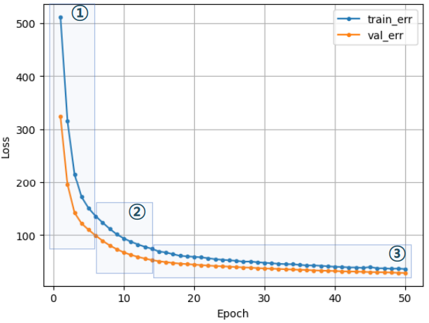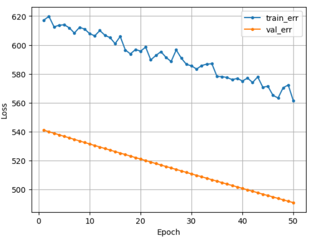① 초기에 오차가 크게 줄고 ② 오차 하락이 꺾임 ③ 점차 완만해짐	case 1 : 학습이 덜 됨, 오차가 줄어들다가 학습이 끝남 ➡️ epoch늘리기, 학습율을 크게 case 2 : train_err가 들쑥날쑥, 가중치 조정이 세밀하지 않음 ➡️ 조금씩 업뎃, 학습율을 작게 case 3 : 과적합, train은 줄어드는데 val은 커짐 ➡️ epoch 수 줄이기

딥러닝 모델링

#라이브러리
import pandas as pd
import numpy as np
import matplotlib.pyplot as plt
import seaborn as sns

from sklearn.model_selection import train_test_split
from sklearn.metrics import *
from sklearn.preprocessing import MinMaxScaler

from keras.models import Sequential
from keras.layers import Dense, Input
from keras.backend import clear_session
from keras.optimizers import Adam

#데이터 준비
target = 'Sales'
x = data.drop(target, axis=1)
y = data.loc[:, target]

#가변수화
cat_cols = ['ShelveLoc', 'Education', 'US', 'Urban']
x = pd.get_dummies(x, columns = cat_cols, drop_first = True)

#데이터분할
x_train, x_val, y_train, y_val = train_test_split(x, y, test_size=.2, random_state = 20)

#전처리
scaler = MinMaxScaler()
x_train = scaler.fit_transform(x_train)
x_val = scaler.transform(x_val)

#모델 선언
nfeatures = x_train.shape[1] #num of columns
nfeatures

# 메모리 정리
clear_session()

# Sequential 타입 모델 선언
model = Sequential([Input(shape = (nfeatures,)),
                    Dense(18, activation = 'relu' ),
                    Dense(4, activation='relu') ,
                    Dense(1) ] )
# 모델요약
model.summary()
#컴파일 
model.compile(optimizer= Adam(learning_rate = 0.1), loss='mse')

#학습, 예측
history = model.fit(x_train, y_train, epochs = 50, validation_split=0.2).history

#검증
pred = model.predict(x_val)
print(mean_squared_error(y_val, pred, squared = False))
print(mean_absolute_error(y_val, pred))
print(mean_absolute_percentage_error(y_val, pred))

학습 그래프 확인

def dl_history_plot(history):
    plt.figure(figsize=(10,6))
    plt.plot(history['loss'], label='train_err', marker = '.')
    plt.plot(history['val_loss'], label='val_err', marker = '.')

    plt.ylabel('Loss')
    plt.xlabel('Epoch')
    plt.legend()
    plt.grid()
    plt.show()
    
#그래프 확인    
dl_history_plot(history)