비지도학습(Unsupervised Learning) 클러스터링(Clustering) - (2) DBSCAN

DBSCAN(Density Based Spatial Clustering of Applications with Noise)이란?

가장 널리 알려진 밀도(density) 기반의 군집 알고리즘이다. 지난 포스팅에서 언급한 K-means 알고리즘을 사용하여 해결하기 어려웠던 문제들을 DBSCAN 알고리즘을 활용해 해결할 수 있다.

🧩 DBSCAN 알고리즘의 특징

• 군집의 개수, 즉 K-means 알고리즘에서의 K 값을 미리 지정할 필요가 없다.
• 유클리드 거리 기반의 K-means 알고리즘 방식과 달리, 조밀하게 몰려 있는 클러스터를 군집화하는 방식을 사용하기 때문에 원 모양이 아닌 불특정한 형태의 군집도 있다.
• 클러스터가 최초의 임의의 점 하나로부터 점점 퍼져나가는데 그 기준이 바로 일정 반경 안의 데이터의 개수, 즉 데이터의 밀도이다.
  출처: http://primo.ai/index.php?title=Density-Based_Spatial_Clustering_of_Applications_with_Noise_(DBSCAN)

1. DBSCAN 알고리즘의 동작

⚓️ K-means에서 K 값 미리 지정, DBSCAN에서는 epsilon과 minPts 값이 미리 지정해야 함!! ⚓️

• epsilon: 클러스터의 반경
• minPts: 클러스터를 이루는 개체의 최솟값
• core point: 반경 epsilon 내에 minPts 개 이상의 점이 존재하는 중심점
• border point: 군집의 중심이 되지는 못하지만, 군집에 속하는 점
• noise point: 군집에 포함되지 못하는 점

1. 임의의 점 p를 설정하고, p를 포함하여 주어진 클러스터의 반경(epsilon) 안에 포함되어 있는 점들의 개수를 센다.
2. 만일 해당 원에 minPts 개 이상의 점이 포함되어 있으면, 해당 점 p를 core point로 간주하고 원에 포함된 점들을 하나의 클러스터로 묶는다.
3. 해당 원에 minPts개 미만의 점이 포함되어 있으면, 일단 pass 한다.
4. 모든 점에 대하여 돌아가면서 1~3 번의 과정을 반복하는데, 만일 새로운 점 p'가 core point가 되고 이 점이 기존의 클러스터(p를 core point로 하는)에 속한다면, 두 개의 클러스터는 연결되어 있다고 하며 하나의 클러스터로 묶어준다.
5. 모든 점에 대하여 클러스터링 과정을 끝낸 후, 어떤 점을 중심으로 하든 클러스터에 속하지 못하는 점은 noise point로 간주해야 한다. 또한, 특정 군집에는 속하지만 core point가 아닌 점들을 border point라 한다.

2. DBSCAN 알고리즘을 적용해보기

# DBSCAN으로 circle, moon, diagonal shaped data를 군집화한 결과
from sklearn.cluster import DBSCAN

fig = plt.figure()
ax= fig.add_subplot(1, 1, 1)
color_dict = {0: 'red', 1: 'blue', 2: 'green', 3:'brown',4:'purple'} # n 번째 클러스터 데이터를 어떤 색으로 도식할 지 결정하는 color dictionary

# 원형 분포 데이터 plot
epsilon, minPts = 0.2, 3 # 2)와 3) 과정에서 사용할 epsilon, minPts 값을 설정
circle_dbscan = DBSCAN(eps=epsilon, min_samples=minPts) # 위에서 생성한 원형 분포 데이터에 DBSCAN setting
circle_dbscan.fit(circle_points) # 3) ~ 5) 과정을 반복
n_cluster = max(circle_dbscan.labels_)+1 # 3) ~5) 과정의 반복으로 클러스터의 수 도출

print(f'# of cluster: {n_cluster}')
print(f'DBSCAN Y-hat: {circle_dbscan.labels_}')

# DBSCAN 알고리즘의 수행결과로 도출된 클러스터의 수를 기반으로 색깔별로 구분하여 점에 색칠한 후 도식
for cluster in range(n_cluster):
    cluster_sub_points = circle_points[circle_dbscan.labels_ == cluster]
    ax.scatter(cluster_sub_points[:, 0], cluster_sub_points[:, 1], c=color_dict[cluster], label='cluster_{}'.format(cluster))
ax.set_title('DBSCAN on circle data')
ax.set_xlabel('X')
ax.set_ylabel('Y')
ax.legend()
ax.grid()

# of cluster: 2
DBSCAN Y-hat: [0 0 1 0 0 0 0 1 1 1 0 1 0 1 1 1 0 0 0 0 0 0 1 1 0 1 1 1 1 0 1 1 0 1 0 1 0
 0 1 0 0 1 0 0 0 1 1 1 0 0 1 1 0 1 1 0 1 1 0 0 0 1 0 0 0 1 1 0 0 0 0 0 1 1
 1 0 1 0 1 0 0 1 1 1 0 0 1 0 0 1 1 1 1 1 1 1 1 0 0 1]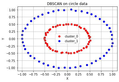

# 달 모양 분포 데이터 plot - 위와 같은 과정 반복
fig = plt.figure()
ax= fig.add_subplot(1, 1, 1)
color_dict = {0: 'red', 1: 'blue', 2: 'green', 3:'brown',4:'purple'} # n 번째 클러스터 데이터를 어떤 색으로 도식할 지 결정하는 color dictionary

epsilon, minPts = 0.4, 3
moon_dbscan = DBSCAN(eps=epsilon, min_samples=minPts)
moon_dbscan.fit(moon_points)
n_cluster = max(moon_dbscan.labels_)+1

print(f'# of cluster: {n_cluster}')
print(f'DBSCAN Y-hat: {moon_dbscan.labels_}')

for cluster in range(n_cluster):
    cluster_sub_points = moon_points[moon_dbscan.labels_ == cluster]
    ax.scatter(cluster_sub_points[:, 0], cluster_sub_points[:, 1], c=color_dict[cluster], label='cluster_{}'.format(cluster))
ax.set_title('DBSCAN on moon data')
ax.set_xlabel('X')
ax.set_ylabel('Y')
ax.legend()
ax.grid()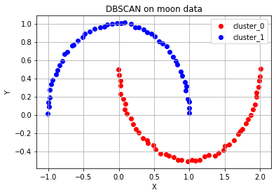

# 대각선 모양 분포 데이터 plot - 위와 같은 과정 반복
fig = plt.figure()
ax= fig.add_subplot(1, 1, 1)
color_dict = {0: 'red', 1: 'blue', 2: 'green', 3:'brown',4:'purple'} # n 번째 클러스터 데이터를 어떤 색으로 도식할 지 결정하는 color dictionary

epsilon, minPts = 0.7, 3
diag_dbscan = DBSCAN(eps=epsilon, min_samples=minPts)
diag_dbscan.fit(diag_points)
n_cluster = max(diag_dbscan.labels_)+1

print(f'# of cluster: {n_cluster}')
print(f'DBSCAN Y-hat: {diag_dbscan.labels_}')

for cluster in range(n_cluster):
    cluster_sub_points = diag_points[diag_dbscan.labels_ == cluster]
    ax.scatter(cluster_sub_points[:, 0], cluster_sub_points[:, 1], c=color_dict[cluster], label='cluster_{}'.format(cluster))
ax.set_title('DBSCAN on diagonal shaped data')
ax.set_xlabel('X')
ax.set_ylabel('Y')
ax.legend()
ax.grid()

# of cluster: 3
DBSCAN Y-hat: [ 0  1  1  0  0  2  2  0  1  2  2  2  0  2  0  1  2  2  2  1  1  1  1  1
  2  2  0  1  0  2  1  0  2  1  2  0  0  0  0  0  1  0  1  0  0  2  1  1
  0  2  1  1  2  1  0  2 -1  2  0  0  2  0  0  1  0  1  1  2  2  2 -1  0
  2  0  0  0  1  2  2 -1  2  2  1  2  0  0  2  1  1  2  1  1  2  0 -1  1
  0  0  0  1]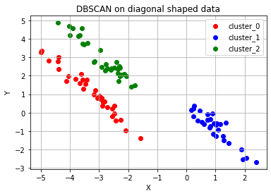

🧩 DBSCAN Y-hat 결과가 -1인 경우 어느 군집에도 포함되지 못한 noise point 가 존재한다는 뜻.

epsilon과 minPts 값을 잘 조절해 주면 DBSCAN 알고리즘에 따라 클러스터의 수를 명시해 주지 않아도 적절한 클러스터의 개수를 설정하여 주어진 데이터에 대한 군집화를 수행할 수 있다. 클러스터의 수를 지정해 주고, 데이터의 분포를 신경 써야 하는 K-means 알고리즘에 비해 훨씬 유연한 사용이 가능하기 때문에 DBSCAN은 굉장히 보편적으로 사용되는 군집화 알고리즘이다.

3. DBSCAN 알고리즘과 K-means 알고리즘의 소요 시간 비교

# DBSCAN 알고리즘과 K-means 알고리즘의 시간을 비교하는 코드 
import time

n_samples= [100, 500, 1000, 2000, 5000, 7500, 10000, 20000, 30000, 40000, 50000]

kmeans_time = []
dbscan_time = []
x = []
for n_sample in n_samples:
    dummy_circle, dummy_labels = make_circles(n_samples=n_sample, factor=0.5, noise=0.01) # 원형의 분포를 가지는 데이터 생성

    # K-means 시간을 측정
    kmeans_start = time.time()
    circle_kmeans = KMeans(n_clusters=2)
    circle_kmeans.fit(dummy_circle)
    kmeans_end = time.time()

    # DBSCAN 시간을 측정
    dbscan_start = time.time()
    epsilon, minPts = 0.2, 3
    circle_dbscan = DBSCAN(eps=epsilon, min_samples=minPts)
    circle_dbscan.fit(dummy_circle)
    dbscan_end = time.time()

    x.append(n_sample)
    kmeans_time.append(kmeans_end-kmeans_start)
    dbscan_time.append(dbscan_end-dbscan_start)
    print("# of samples: {} / Elapsed time of K-means: {:.5f}s / DBSCAN: {:.5f}s".format(n_sample, kmeans_end-kmeans_start, dbscan_end-dbscan_start))

# K-means와 DBSCAN의 소요 시간 그래프화
fig = plt.figure()
ax = fig.add_subplot(1, 1, 1)
ax.scatter(x, kmeans_time, c='red', marker='x', label='K-means elapsed time')
ax.scatter(x, dbscan_time, c='green', label='DBSCAN elapsed time')
ax.set_xlabel('# of samples')
ax.set_ylabel('time(s)')
ax.legend()
ax.grid()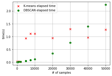

DBSCAN의 단점은?

• 보시다시피, 데이터의 수가 적을 때는 K-means 알고리즘의 수행 시간이 DBSCAN에 비해 더 길었으나, 군집화할 데이터의 수가 많아질수록 DBSCAN의 알고리즘 수행 시간이 급격하게 늘어난다.
• 클러스터의 수를 지정해 줄 필요가 없으나 데이터 분포에 맞는 epsilon과 minPts의 값을 지정해 주어야 한다.