s1 <- c(1, 2, 1, 2, 3, 4, 2, 3, 4, 5)
s2 <- c(1, 3, 1, 2, 3, 4, 2, 4, 3, 4)
s3 <- c(2, 3, 2, 3, 2, 3, 5, 3, 4, 2)
s4 <- c(2, 4, 2, 3, 2, 3, 5, 3, 4, 1)
s5 <- c(4, 5, 4, 5, 2, 1, 5, 2, 4, 3)
s6 <- c(4, 3, 4, 4, 2, 1, 5, 2, 4, 2)
name <- 1:10
subject <- data.frame(s1, s2, s3, s4, s5, s6)
str(subject)
pc <- prcomp(subject)
summary(pc)
plot(pc)
prcomp(subject)
en <- eigen(cor(subject))
names(en)
en$values
en$vectors
plot(en$values, type = "o")
cor(subject)
result <- factanal(subject, factors = 2, rotation = "varimax")
result
result <- factanal(subject,
factor = 3,
rotation = "varimax",
scores = "regression")
result
attributes(result)
result$loadings
print(result, digits = 2, cutoff = 0.5)
print(result$loadings, cutoff = 0)
plot(result$scores[ , c(1:2)],
main = "Factor1과 Factor2 요인점수 행렬")
text(result$scores[ , 1], result$scores[ , 2],
labels = name, cex = 0.7, pos = 3, col = "blue")
points(result$loadings[ , c(1:2)], pch = 19, col = "red")
text(result$loadings[ , 1], result$loadings[ , 2],
labels = rownames(result$loadings),
cex = 0.8, pos = 3, col = "red")
plot(result$scores[ , c(1, 3)],
main = "Factor1과 Factor3 요인점수 행렬")
text(result$scores[ , 1], result$scores[ , 3],
labels = name, cex = 0.7, pos = 3, col = "blue")
points(result$loadings[ , c(1, 3)], pch = 19, col = "red")
text(result$loadings[ , 1], result$loadings[ , 3],
labels = rownames(result$loadings),
cex = 0.8, pos= 3, col = "red")
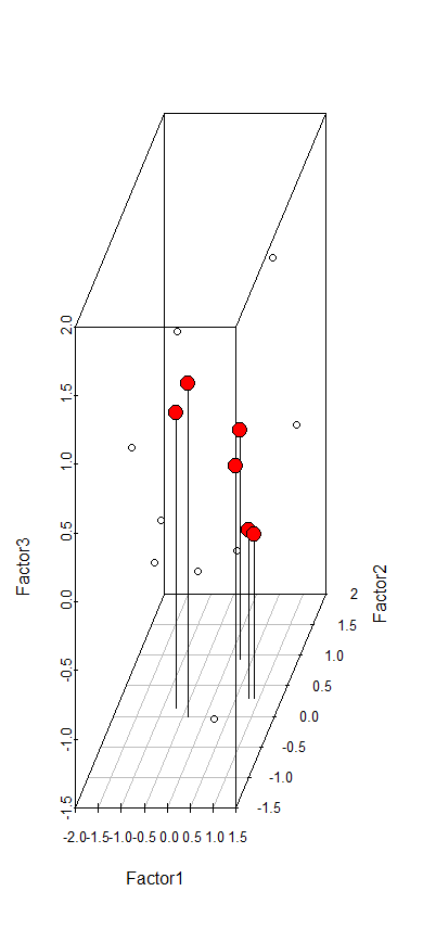
library(scatterplot3d)
Factor1 <- result$scores[ , 1]
Factor2 <- result$scores[ , 2]
Factor3 <- result$scores[ , 3]
d3 <- scatterplot3d(Factor1, Factor2, Factor3, type = 'p')
loadings1 <- result$loadings[ , 1]
loadings2 <- result$loadings[ , 2]
loadings3 <- result$loadings[ , 3]
d3$points3d(loadings1, loadings2, loadings3,
bg = 'red', pch = 21, cex = 2, type = 'h')
app <- data.frame(subject$s5, subject$s6)
soc <- data.frame(subject$s3, subject$s4)
nat <- data.frame(subject$s1, subject$s2)
app_science <- round((app$subject.s5 + app$subject.s6) / ncol(app), 2)
soc_science <- round((soc$subject.s3 + soc$subject.s4) / ncol(soc), 2)
nat_science <- round((nat$subject.s1 + nat$subject.s2) / ncol(net), 2)
subject_factor_df <- data.frame(app_science, soc_science, nat_science)
cor(subject_factor_df)
library(memisc)
setwd("C:/Rwork/ ")
data.spss <- as.data.set(spss.system.file('drinking_water.sav'))
data.spss[1:11]
drinking_water <- data.spss[1:11]
drinking_water_df <- as.data.frame(data.spss[1:11])
str(drinking_water_df)
result2 <- factanal(drinking_water_df, factor = 3, rotation = "varimax")
result2
dw_df <- drinking_water_df[-4]
str(dw_df)
dim(dw_df)
s <- data.frame(dw_df$Q8, dw_df$Q9, dw_df$Q10, dw_df$Q11)
c <- data.frame(dw_df$Q1, dw_df$Q2, dw_df$Q3)
p <- data.frame(dw_df$Q5, dw_df$Q6, dw_df$Q7)
satisfaction <- round(
(s$dw_df.Q8 + s$dw_df.Q9 + s$dw_df.Q10 + s$dw_df.Q11) / ncol(s), 2)
closeness <- round(
(c$dw_df.Q1 + c$dw_df.Q2 + c$dw_df.Q3) / ncol(s), 2)
pertinence <- round(
(p$dw_df.Q5 + p$dw_df.Q6 + p$dw_df.Q7) / ncol(s), 2)
drinking_water_factor_df <- data.frame(satisfaction, closeness, pertinence)
colnames(drinking_water_factor_df) <- c("제품만족도", "제품친밀도", "제품적절성")
cor(drinking_water_factor_df)
length(satisfaction); length(closeness); length(pertinence)