RTMDet

• Real-time instance segmentation에서 좋은 성능
  • convolutional object detectors VS Vision transformer 계열
    • 전자가 Real-time application에 적합하여, 많이 쓰이고 있음.
• https://arxiv.org/pdf/2212.07784.pdf

---

Abstract

• YOLO 시리즈보다 real-time object detection 잘함
• instance segmentation 과 같은 tasks에 쉽게 확장 가능
  • segmentation task는 detection task에 비해, output feature resolution이 너무 작으면 성능이 떨어집니다.
• architecture
  • 아래의 구조 덕분에, backbone 과 neck에 호환 가능한 capacity를 가진 architecture를 제안(한 부분이 다른 부분의 성능이나 용량에 제한을 받지 않도록 고려된 구조)
    • large-kernel depth-wise convolutions로 구성된 basic building block (backbone과 neck모두 같은 basic building block을 씀)
    • depth-wise convolution 개념과 쓰는 이유: https://velog.io/@hsbc/depth-wise-separable-convolution
• soft labels 제안
  • (dynamic label assignment 문제에서,) matching cost를 계산할 때 soft labels를 도입함으로써, 정확도를 높임
• 최고의 parameter-accuracy trade-off
• real-time instance segmentation에서 SOTA!

---

그림

그림 1

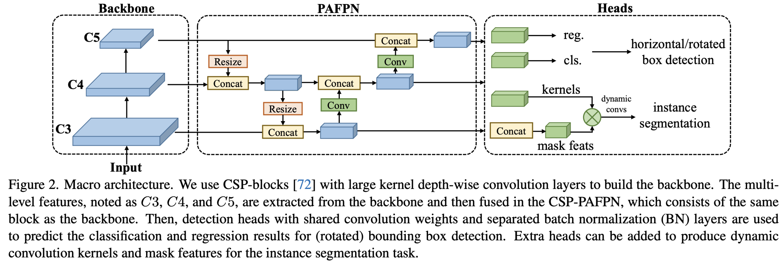
Backbone:

• CSP-block[72]를 사용
  • https://velog.io/@hsbc/CSPCross-Stage-Partial-Net
  • CSP block + large-kernel depth-wise convolution layers의 조합

PAFPN (Panoptic Feature Pyramid Network)

• backbone과 같은 block을 사용
• 이 네트워크는 다양한 크기의 객체를 탐지하기 위해 서로 다른 크기의 특징 맵을 결합합니다.
• encoder-decoder 깊이의 영향: https://velog.io/@hsbc/Encoderdecoder-깊이의-영향

Heads

• box regression / classification
  • shared convolution weight and separated batch normalization layers

---

그림 2

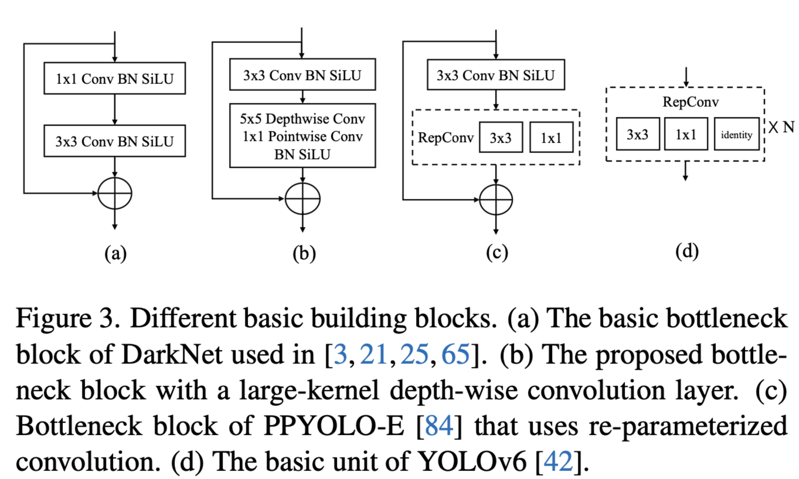
a

• a는 YOLO 계열에서 많이 쓰임
• 4 depth

b

• b가 논문에서 제안하는 것 = a에서 inference speed 개선 (계산량이 줄어듦)
  • b의 2번째 block을 depthwise separable convolution이라 부르기도 함
    • https://velog.io/@hsbc/depth-wise-separable-convolution
    • depthwise separable convolution 장점: weight 수가 적은데(메모리 적게 사용), 성능이 좋다.
  • 하지만, weight 수를 줄이는 부작용으로 inference speed 측면(계산량)에서 단점이 생겨버림 (1*1 point-wise convolution이 추가되어서) -> 이를 해결하기 위해
    • depth를 3으로 줄임. but, depth를 줄이면서 생긴, 작은 물체(디테일)을 잡아내는 능력이 떨어지는 부작용을 해결하기 위해
      • width of block(output channel 수)는 늘림.
• 결론적으로는, a와 성능은 같으면서도, inference speed를 빠르게 할 수 있었다.

c, d

• 어떤 최근 연구들은, re-parameterized convolution을 썼다. (장단점도 아래 글에 적혀있음)
  • (TODO) https://velog.io/@hsbc/reparameterized-convolution

---

그림 3

• 

---

Method

3.2 Model architecture

Basic Building Block

• 과거에는 계산량을 줄이면서도 성능을 유지하기 위해 dilated convolution이나 Non-local neural networks 등을 이용했지만, 이것조차 real-time에 쓰기엔 부족하였다.
• 최근 연구들은, real-time 목적 달성을 위해, large-kernel depth-wise convolution을 쓰는게 트렌드다.

Balance of model width and depth

• 그림 2 참조.

Balance of backbone and network

• multi-scale feature 성능 향상을 위해 (물체 크기와 무관하게 성능을 높이기 위해)
  • 과거에는
    • larger backbone을 쓰거나, heavier neck을 썼는데
  • 내 논문은
    • neck의 basic block에 expansion ratio를 높임으로써 -> computation-accuracy trade-off를 개선하였다.
      • Expansion ratio가 뭘까? : neck basic block의 output의 channel 수를 늘린다는 뜻인가?

Shared detection head

• parameter 개수를 줄이면서, 성능을 유지한 head!
  • 과거의 real-time object detector head
    • different feature scale 마다 seperate detection heads를 사용함.
  • 우리는
    • (TODO) multiple scale 마다 shared parameter head를 썼고,
    • 그 대신, scale마다 다른 BN layer을 둠
      • BN은 GN 과 같은 다른 normalization layer보다도 더 효율적인데, 그 이유는
        • inference 시에, training 시 계산된 통계를 바로 사용할 수 있기 때문이다.
      • normalization layer: https://velog.io/@hsbc/normalization-layers

3.3 Training Strategy

Label assignment and losses

• 1-stage detector VS 2-stage detector: https://velog.io/@hsbc/one-stage-detector-VS-two-stage-detector
• 2-stage는 localization먼저 하고 -> 해당 box의 이미지 classify를 진행한다.
• 하지만 1-stage는 localization과 classify를 동시에 진행
  • 각 scale로부터의 dense predictions이 ground truth bounding box와 매칭되어야 함.
  • 이떄 이용하는 것이 label assignment strategies [19, 47, 70]
  • https://velog.io/@hsbc/Label-Assignment-Strategy
• 최근 연구들은 dynamic label assignment strategies를 사용 [6, 20, 21]
  • https://velog.io/@hsbc/dynamic-label-assignment
  • 하지만: cost calculation에 문제가 있었다.
• [논문이 제안] dynamic soft label assignment strategy
• 

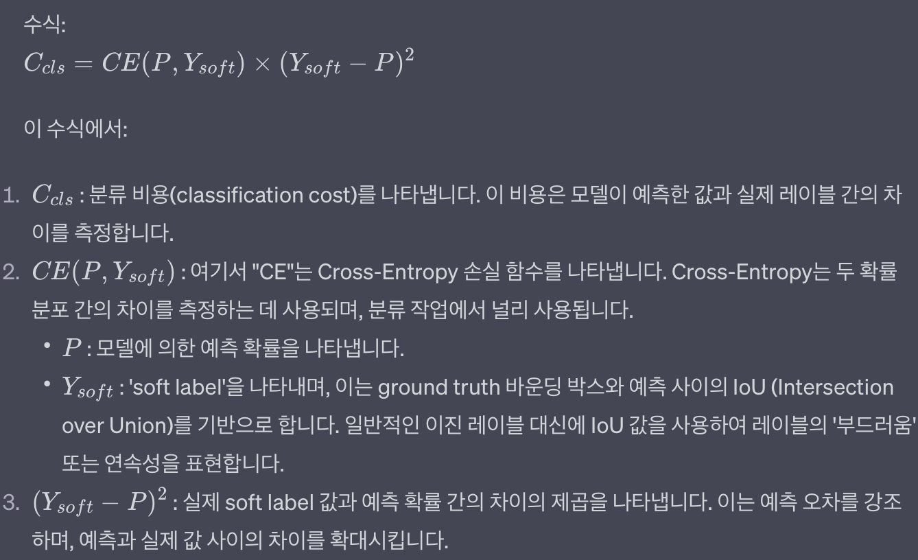
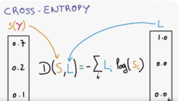
cls loss

• 과거 논문에서는 binary labels(매칭 됐냐 or 안 됐냐 기반)를 이용해서 cls loss를 계산함. 하지만 아래의 문제가 있었음.
  • classification 성능과 bounding box regression 성능이 서로 방해를 함.
• 우리 cls loss는 (binary label로 인해,) noisy하고 unstable하게 학습되는 것을 막습니다.
• Y_soft: IoU = soft label
• regression quality에 따라, classification loss를 reweight 합니다.
  • IOU가 작으면, 고양이라고 추측할 확률을 좀 더 낮게 학습
  • IOU가 크면, 고양이라고 추측할 확률을 좀 더 높게 학습
    • IOU가 1이면, Y_soft는 1이 됨
• 
• 

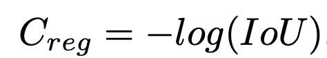
Regression loss

• Generalized IOU[67] 대신, 아래를 사용
  • GIOU의 단점: maximum difference between the best match and the worst match is less than 1
• 그 이유는, IOU가 틀렸을 떄, 더 큰 cost를 주기 위함
• 

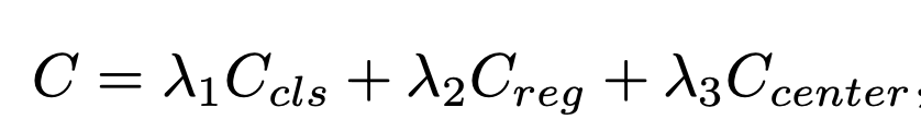
center loss

• soft center region cost
• 
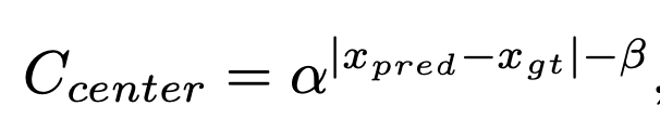
• α and β are hyper-parameters of the soft center re-
  gion. We set α = 10, β = 3 by default.

Cached Mosaic and MixUp

• 최근 object detection area에서 널리 쓰이고 있는 cross-sample augmentation 방법론들: MixUp , CutMix
  • https://velog.io/@hsbc/Cross-sample-augmentation
• 위 2가지 방법의 2가지 side effect
  • each iteration 마다, training sample을 만들기 위해 multiple images를 load하는 것이 필요함.
    • data loading cost가 들어. -> 그래서 학습을 느리게 함.
  • 생성된 training sample이 noisy 해서, 실제 data distribution과 맞지 않을 수 있다.
• 제안
  • MixUp과 Mosaic을, caching mechanism 을 통해 개선함. (data loading cost를 줄임)
    • training pipeline에서의 mixing image cost가 매우 감소함.
    • cache operation: cache length와 popping method에 의해 제어
      • large cache length + random popping: 기존의 MixUP과 Mosaic과 비슷
      • small cache length + FIFO popping: repeated augmentation과 비슷

Two-stage training

YOLOX

• To reduce the side effects of ‘noisy’ samples by strong data augmentations, YOLOX [21] explored a two-stage training strategy,
  • where the first stage uses strong data augmentations, including Mosaic, MixUp, and random rotation and shear,
  • and the second stage use weak data augmentations, such as random resizing and flipping.
  • As the strong augmentation in the initial training stage includes random rotation and shearing that cause misalignment between inputs and the transformed box annotations,
    • YOLOX adds the L1 loss to fine-tune the regression branch in the second stage.
  • To decouple the usage of data augmentation and loss functions,
    • we exclude these data augmentations and increase the number of mixed images to 8 in each training sample in the first training stage of 280 epochs to compensate for the strength of data augmentation.
    • In the last 20 epochs, we switch to Large Scale Jittering (LSJ) [22],
      • allowing for fine-tuning of the model in a domain that is more closely aligned with the real data distributions.
    • To further stabilize the training, we adopt AdamW [55] as the optimizer,
      • which is rarely used in convolutional object detectors but is a default for vision transformers [16].

3.4 Extending to other tasks

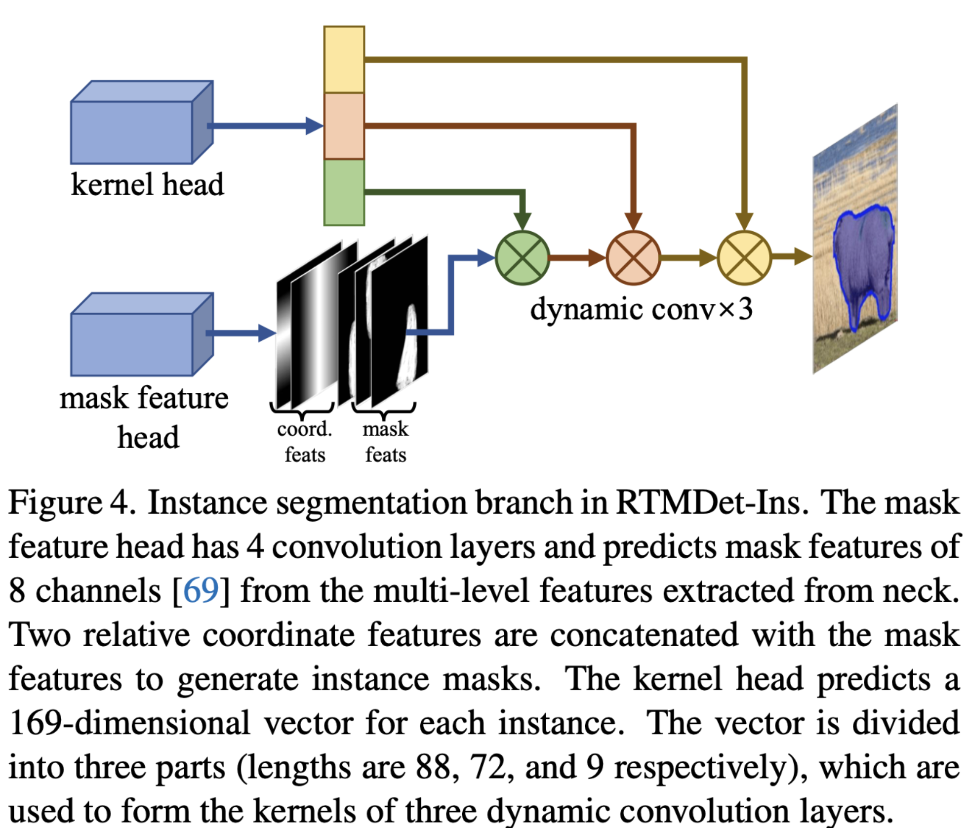
Instance segmentation

• The mask feature head
  • 4 convolution layers
  • extract mask features with 8 channels from multi-level features.
• kernel prediction head
  • 각 instance마다 169 차원 벡터를 예측
  • 169 차원 벡터는 three dynamic convolution kernels 로 분해
    • mask features and coordinate features와 결합하여, instance segmentation masks 생성
• mask annotations에 내재된 사전 정보를 더 잘 이용하기 위해, 우리는 soft region prior in the dynamic label assignment를 계산 할 때
  • box center 대신, mass center of the masks를 사용함.
• dice loss 사용: https://velog.io/@hsbc/dice-loss-사용

---