Info

• paper : Fast R-CNN
• author : Ross Girshick
• subject : Girshick, Ross. "Fast r-cnn." Proceedings of the IEEE international conference on computer vision. 2015.

사전지식 : R-CNN, SPPnet

• R-CNN ➡️ SPPnet ➡️ Fast R-CNN ➡️ Faster R-CNN
  • R-CNN simple review : https://velog.io/@hseop/Simple-Review-Region-based-Convolutional-Networks-for-Accurate-Object-Detection-and-Segmentation
  • SPPnet 내용 파악을 위해 읽은 paper review :
    https://velog.io/@twinjuy/SPPNet-%EB%85%BC%EB%AC%B8-%EB%A6%AC%EB%B7%B0Spatial-Pyramid-Pooling-Network

요약) R-CNN의 단점
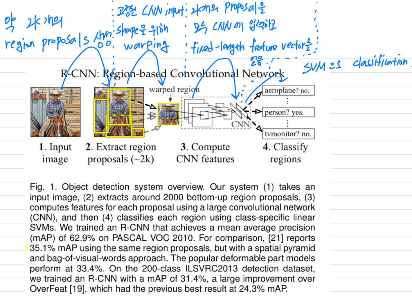
1. 한 image에 대해서 selective search로 2,000개의 proposal(candidate)를 뽑고 나서
각각의 candidate마다 CNN model을 적용하기 때문에 시간이 매우 오래 걸림
2. CNN, SVM, Bounding Box Regression을 총 세가지 model이 multi-stage pipeline이고,
또한 SVM, Bounding Box Regression이 CNN을 학습시키지 못하기 때문에 end-to-end 학습이 되지 않음.

➡️ R-CNN의 주요한 두가지 단점을 극복하기 위해 RoI pooling을 사용한 Fast R-CNN이 나옴

---

Abstract

• Fast R-CNN은 deep convolutional networks를 사용하여
  previous work에 대해 효율적으로 object proposal을 classify하는 model로 만듦.

• previous work와 비교하여,
  Fast R-CNN은 detection accuracy를 상승시키면서
  training and testing speed를 향상시킨
  몇 가지 innovations를 사용했다.

• Fast R-CNN은 R-CNN보다 9배 빠른 VGG16을 train시키고,
  test-time에는 213배 빨랐다.
  그리고 PASCAL VOC 2012에 대해 더 높은 mAP를 달성했다.

---

1. Introduction

• 최근 deep ConvNet은 image classification과 object detection 분야에 엄청난 발전을 일으키고 있다.

• image classification과 비교하여 object detection은
  해결하기 위해 더욱 complex methods가 필요하기 때문에 더욱 challenging task라고 할 수 있다.

• detection은 object에 대한 정확한 localization이 필요하기 때문에 complexity가 상승한다.
  또한 두 가지 주요한 challenge가 있다.

  1. "proposals"이라고 불리는 매우 많은 candidate object locations가 처리되어야 한다.
  2. 이러한 candidates들은 정확한 localization을 위해 다시 refine해야만 하는 대략적인 localization을 제공한다.
     
     이 문제들에 대한 solution은 speed, accuracy, simplicity를 타협한다.

• 이 논문에서, 우리는 state-of-the-art ConvNet based의 object detector의 training process를 간소화했다.
  우리는 object proposals(=candidates)를 classification하고, proposals의 spatial locations을 refine(정제)하는 것을
  함께 학습할 수 있는 a single-stage training algorithm을 제안할 것이다.

1.1. R-CNN and SPPnet

• The Region-based Convolutional Network method(R-CNN)은 훌륭한 object detection accuracy를 달성했지만,
  명백한 drawbacks을 갖는다 :
  1. Training is a multi-stage pipeline.
     • R-CNN은 처음에 log loss를 이용하여 object proposals에 대한 ConvNet을 finetune한다.
     • 그리고나서, ConvNet feature들을 SVMs에 fit한다.
       SVM들은 object detectors처럼 작동한다.
     • 세번째 training stage에서는, bounding-box regressor들이 학습되어진다.
  2. Training is expensive in space and time.
     • SVM과 bounding-box regressor training을 위해서,
       feature들은 각 image의 각각 object proposal들로부터 추출되어져야 하고,
       disk에 write되어져야 한다.
     • VGG16과 같은 deep networks에서는 5K의 VOC07 trainval set을 위해 2.5 GPU-days가 걸린다.
       이 feature들은 storage의 수백 gigabytes가 필요하다.
  3. Object detection is slow.
     • test-time에, feature들은 각각의 test iamge의 각각의 object proposal로부터 feature들이 추출되어진다.
     • Nvidia K40 GPU를 사용하여 VGG16에서 detection은 47s / image 이다.
       (한 image 당 feature extraction에 47초가 소요된다)
• 이렇듯,
  R-CNN은 각각의 object proposal에 대한 ConvNet forward pass가 computation sharing 없이 진행되기 때문에 느리다.
  
  

1.2. Contributions

• 우리는 R-CNN의 단점을 고치며 speed와 accuracy를 향상시킬 수 있는 새로운 training algorithm을 제안한다.
• 우리는 이 method를 R-CNN보다 train과 test가 비교적 빠르기 때문에
  Fast R-CNN이라고 부른다.
• The Fast R-CNN method는 여러가지 장점이 있다 :
  1. High detection quality(mAP) than R-CNN, SPPnet
  2. Training is single-stage, using a multi-task loss
  3. Training can update all network layers
  4. No disk storage is required for feature caching

---

2. Fast R-CNN architecture and training

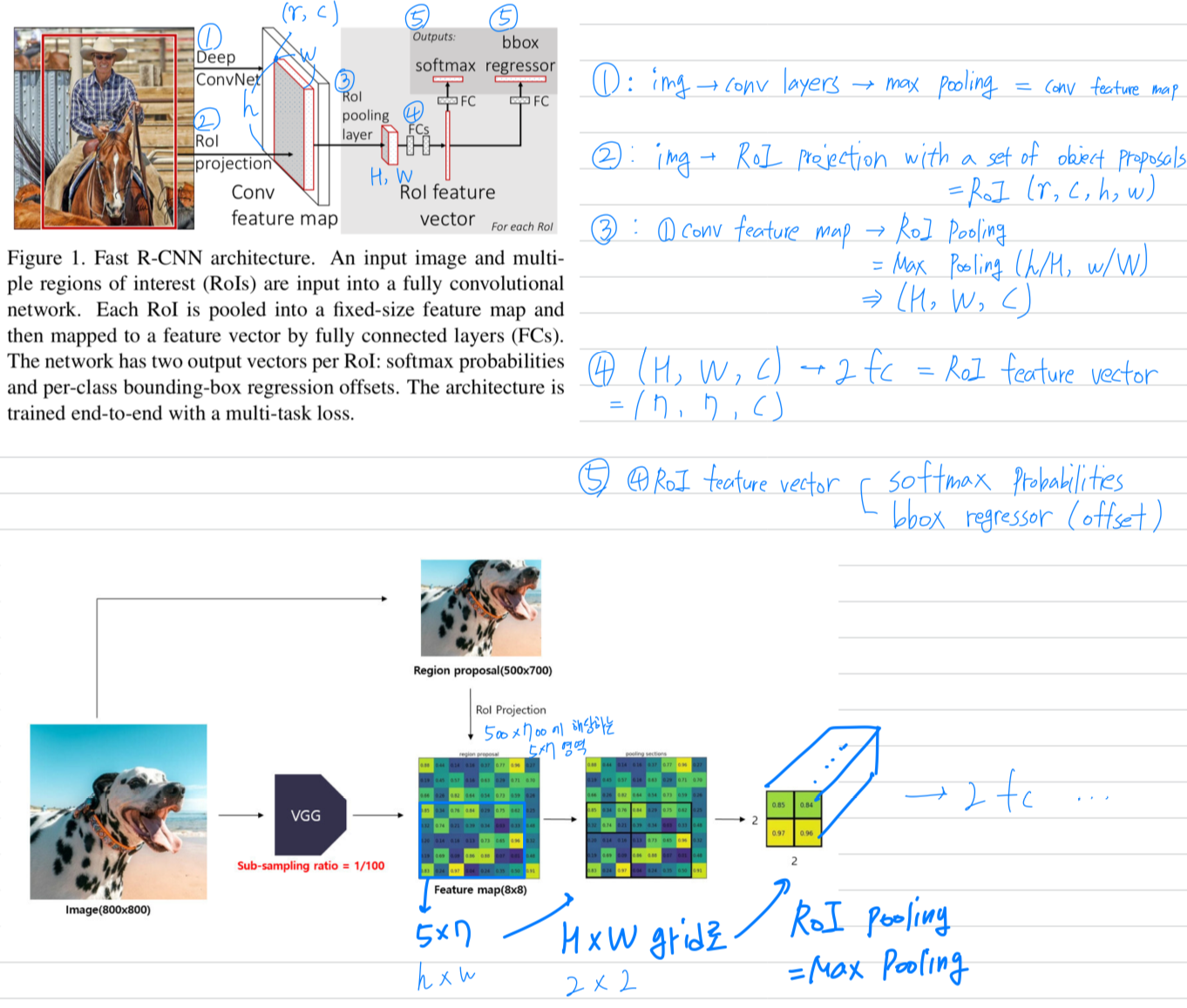
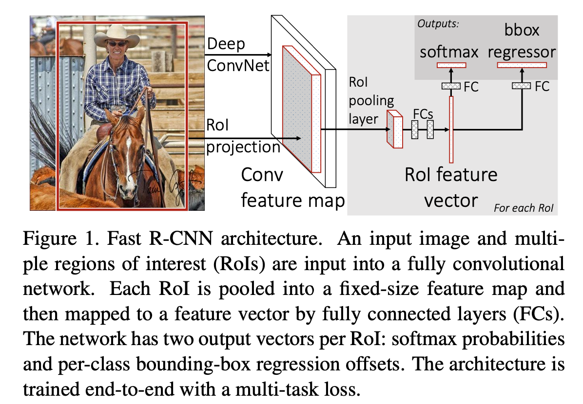
• Fig. 1에 Fast R-CNN architecture를 설명하고 있다.
  • Fast R-CNN network는
    entire image와 a set of object proposals을 input으로 갖는다.
  • Fast R-CNN network는
    전체 image에 대해 several conv layer를 거치고,
    max pooling layer를 통해 conv feature map을 생성한다.
  • 그리고 나서 각 object proposal에 대해서,
    a region of interest(RoI) pooling layer는
    feature map으로부터 a fixed-length feature vector를 추출한다.
  • 각각의 feature vector들은 fc layer로 들어가고,
    마침내 2개의 sibling output layer로 나누어진다.
    (1) K개의 object class와 추가적으로 "background(배경)" class에 대한
    softmax probability estimates를 생성.
    (2) 각 K개의 object class에 대한 4개의 실수값을 출력하고,
    each set of 4 values는 K개 class 중 하나에 대한 refine된 bounding-box를 encode.
    

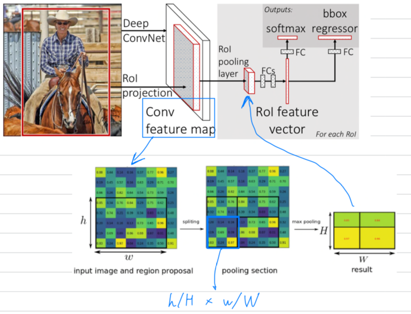
2.1. The RoI pooling layer

• The RoI pooling layer는 max pooling을 사용하여
  유효한 RoI 내의 feature를 a small feature map으로 convert한다.
  이 feature map은 고정된 spatial 크기인 H x W (e.g., 7 x 7)를 가지며,
  여기서 H와 W는 특정 RoI와 독립적인 layer hyper-parameter이다.

• 이 논문에서,
  RoI는 conv feature map에 대한 rectangular window이다.
  rectangular window는 4개의 tuple $(r, c, h, w)$에 의해 정의된다.
  $(r, c)$는 top-left corner, $(h, w)$는 그것의 height와 width를 나타낸다.

• 우선 input image를 CNN에 통과시켜 feature map을 추출하고,
  이전에 미리 selective search로 만들어놨던 RoI를 feature map에 projection시킨다.
  아래 그림의 가장 좌측 그림이 feature map이고, 그 안에 $h$ x $w$는 RoI가 projection된 window이다.
  그리고 미리 설정한 sub-windows의 grid 크기인 $H$ x $W$로 만들어 주기 위해,
  $h$ x $w$를 $H$ x $W$로 나누어,
  $h/H$ x $w/W$로 만든 다음,
  각 sub window를 max-pooling한다.
  
  이제 feature map에 projection했던 $h$ x $w$ size의 RoI는 고정된 $H$ x $W$ size의 a small feature map이 되고,
  이를 feature vector로 convert한다.
  

2.2. Initializing from pre-trained network

• 우리는 5개의 max pooling layer와 5~13개의 conv layer를 가지는 3가지 pre-trained ImageNet network에 대해서 실험을 진행했다.
  (see Section 4.1. for network details) ➡️ 1. CaffetNet(S for "Small"), 2. VGG_CNN_M_1024(M for "Medium"), 3. VGG16(L for "Large"))

• pre-trained network가 Fast R-CNN network를 초기화할 때, 3가지 transformation을 적용했다.

  1. 마지막 max pooling layer를 RoI pooling layer로 바꿨다.
     이 RoI pooling layer는 network의 첫번째 fc layer와 호환되도록 $H$와 $W$를 설정하여 구성되었다.
     (e.g. VGG16을 위해서는 $H$=$W$=$7$)
  2. network의 마지막 fc layer과 softmax는 이전에 설명했던 2가지 sibling layer로 교체되었다.
     1. K+1개의 대한 fc layer의 softmax
     2. category별 bounding-box regressors
  3. network의 두가지 input data가 변경되었다.
     1. a list of images
     2. a list of RoIs in those images

2.3. Fine-tuning for detection

• back-propagation으로 모든 network의 weight를 training시키는 것은 Fast R-CNN의 중요한 능력이다.
  첫번째로, 왜 SPPnet이 spatial pyramid pooling layer에서 weight를 update할 수 없는지 밝혀보겠다.

  • 그 근원은 각 training sample(=RoI)가 다른 image로부터 올 때,
    즉 R-CNN과 SPPnet network가 train되는 방식과 일치하는 경우에,
    SPP layer를 통한 back-propagation은 매우 비효율적이다.
  • 비효율성은 각 RoI가 종종 entire inputi mage를 포함하는 매우 큰 receptive field를 가질 수도 있다는 사실에서 시작된다.
    forward pass가 전체의 receptive field를 처리해야하기 때문에, training inputs은 매우 크다.
    가끔은 entire image가 될 수도 있다.

• 우리는 training 동안 feature sharing의 장점을 갖는 더 효율적인 training method를 제안한다.

  • Fast R-CNN을 training시킬 때,
    stochastic gradient descent(SGD) mini batches를 hierarchical하게 sampling한다.
    • 먼저 $N$개의 image를 sampling하고 나서, 각 image에서 $R/N$개의 RoI를 sampling한다.
      중요한 점은, 동일한 image로부터 나온 RoI가 forward pass와 backward pass에서 computation과 memory를 공유한다는 것이다.
    • $N$을 작게 만들어나가는 것은 mini-batch computation을 감소시킬 수 있다.
      예를 들어, $N=2$와 $R=128$을 사용할 때,
      제안된 training 방법은 128개의 서로 다른 image로부터 1개의 RoI를 sampling하는 것보다(= R-CNN과 SPPnet strategy) 약 64배나 빠르다.

• 이 방법의 한가지 우려는 같은 image로부터 RoI가 연관되어있기 때문에 training convergence가 느려질 것이라는 것이다.
  하지만 실제로 이 우려는 발생하지 않았고,
  우리는 R-CCN보다 더 적은 SGD iterations과 $N=2$ and $R=128$을 이용하여 좋은 결과를 달성했다.

• hierarchical sampling을 추가하여,
  Fast R-CNN은
  R-CNN과 SPPnet에서의 3가지 단계(softmax classifier, SVNs, regressors)를 training하는 것보다
  softmax classifier와 bounding-box regressors를 함께 optimize하는 one fine-tuning stage로 간략화된 training process를 사용한다.

• 이 과정의 구성요소는 아래에 설명되어 있다.

  • Multi-task loss
  • Mini-batch sampling
  • Back-propagation through RoI pooling layers
  • SGD hyper-parameters

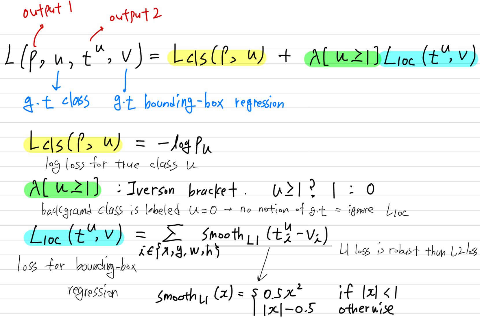
Multi-task loss

• Fast R-CNN은 두 가지 sibling output layer를 갖는다.
  1. 첫 번째 layer의 output은 probability dstribution(per RoI), $p = (p_0, ..., p_K)$, over K+1 categories.
     $p$는 fc layer의 K+1 outputs에 대한 softmax로 계산되어진다.
  2. 두 번째 layer의 output은 bounding-box offsets,
     $t^k = (t_x^k, t_y^k, t_w^k, t_h^k)$, for each of the $K$ object classes, indexed by $k$
• 각각의 training RoI는
  ground-truth class $u$로 label되어지고,
  ground-truth bounding-box target $v$로 label되어진다.
  

Mini-batch sampling

• fine-tuning 동안에,
  각각의 SGD mini-bath들은 uniformly random하게 선택된 $N=2$ images에서 구성된다.
  우리는 크기가 $R=128$인 mini-batch를 사용하여, 각 image에 대해서 64개의 RoI를 sampling한다.

• 우리는 ground truth bounding box와 IoU(Intersection over Union)이 적어도 0.5 이상인 object proposals에서부터 25%의 RoI를 취했다.
  이러한 RoI들은 $u \ge 1$인 foregournd object class로 label되어지는 example들을 형성한다.

• RoI가 $[0.1, 0.5)$인 구간에서 ground truth와 maximum IoU를 갖는 object proposals에서 sampling된다.
  이러한 RoI들은 $u = 0$인 background example이다.

• The lower thhreshold of 0.1 appears to act as a heuristic for hard example mining

  • 예를 들어,
    N = image개수 = 2, R = RoI개수 = 12
    R/N = 64.
    64개의 RoI를 1장의 image에서 sampling.
    여기서 25%(16장)은 ground truth box와의 IoU가 0.5 이상이고 (u >= 1)
    75%(48장)은 ground truth box와의 IoU가 [0.1, 0.5)인 (u == 0) 조건을 적용함.

• training 동안에,
  image들은 probability 0.5로 horizontally flipped되어졌고,
  더 이상의 data augmentation은 없었다.

Back-propagation through RoI pooling layers

(skip했음...)

• Let $x_i \in R$ be the $i$-th activation input into the RoI pooling layer and let $y_{rj}$ be the layer's $j$-th output from the $r$-tg RoI.
  The RoI pooling layer computes $y_{rj}=x_{i*(r,j)}$ ,in which $i*(r,j)=argmax_{i' \in R(r,j)}x_{i'}$.
  $R(r, j)$ is the index set of inputs in the sub-window over which the output unit $y_{rj}$ max pools.
  A single $x_i$ may be assigned to several different outputs $y_{rj}$.

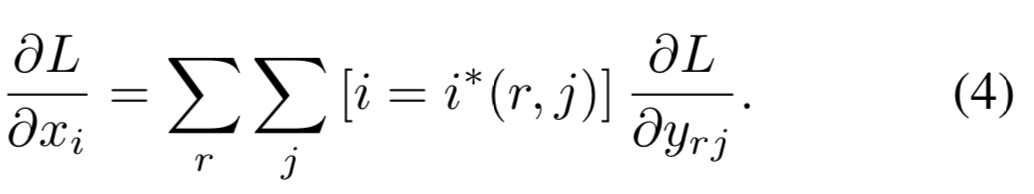
• The RoI pooling layer's backwards function computes partial derivative of the loss function with respect to each input variable $x_i$ by following the argmax switches :
  

SGD hyper-parameters

• softmax classification과 bounding-box regression을 위한 fc layer들은
  각각 standard deviations이 0.01 and 0.001을 갖는 zero-mean Gaussian distributions으로 초기화되어졌다.
• Bias는 모두 0으로 초기화했다.
• 모든 layer에서는 weight에 대한 learning rate 1, bias에 대한 learning rate 2, 그리고 global learning rate를 0.001로 했다.
• VOC07, OVC12 trainval을 훈련시킬때, 우리는 30k mini-batch iteration을 반복 실행한 후 learning rate를 0.0001로 낮추어 추가로 10k iteration을 반복했다.
• momentum은 0.9, parameter decay of 0.0005 가 사용되어졌다.

2.4. Scale invariance

• 우리는 scale invariant object detection을 달성하기 위해 두가지 방법을 실험했다.
  1. brute force :
     brute-force approach에서는 training과 test 중에
     각 image가 사전 정의된 pixel size로 처리됩니다.
     network는 training data에서 직접적으로 scale-invariant object detection을 학습해야 한다.
  2. by using image pyramids
     반면에, multi-scale approach는 image pyramid를 통해 network에 대한 대략적인 scale-invariance을 제공한다.
     test시에, image pyramid는 각 object proposal에 대해 대략적으로 scale-normalize하는 데에 사용된다.
     multi-scale training 동안에는, 우리는 random하게 image가 sampling될 때마다
     data augmentation의 형태로 사용된다.
     우리는 GPU memory 제한으로 인해 multi-scale training은 작은 network에 대해서만 실험했다.

---

3. Fast R-CNN detection

• Fast R-CNN network가 fine-tune되었다면,
  detection은 forward pass를 실행하는 것과 다를게 없다.
  network는 입력으로 image와 점수 매겨질 R개의 object proposal list를 받는다.

• Test time에, R은 일반적으로 약 2000이지만 더 큰 경우도 고려했다.
  image pyramid를 사용할 때,
  각 RoI는 $224^2$ pixel과 가장 근접한 크기로 scaled RoI로 할당되었다.

• 각각의 test RoI $r$애 대해서, forward pass는
  class posterior probability distribution $p$와
  $r$에 의해 예측된 a set of predicted bounding-box offsets을 출력한다.

• 우리는 각 object class $k$에 대해 $r$에 대한 object confidence를 할당하는데,
  estimated probability $Pr(class = k | r) \simeq pk$를 사용했다.
  그리고나서 R-CNN의 algorithm과 setting을 사용하여 각 class에 대해 독립적으로
  non-maximum suppression을 수행했다.

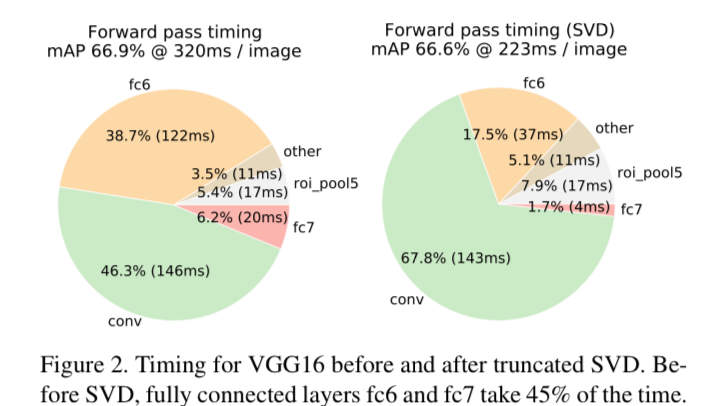
3.1. Truncated SVD for faster detection

• whole-image classification에서,
  fc layer를 computing하는 데에 드는 시간은 conv layer에 비교하여 매우 적습니다.
  반면에 detection에서, 처리하기 위한 RoI의 개수는 매우 많고 fc layer를 computing하기 위해 걸리는 시간은 forward pass에 거의 절반을 차지합니다.
  Large fc layer에서는 truncated SVD를 사용하여 compressing함으로써 쉽게 가속화할 수 있습니다.

• 이 기법에서,
  $u$ x $v$ weight matrix $W$로 parameterized된 layer는
  SVD를 이용하여 대략적으로 factorize시킬 수 있습니다.
  $U$는 $W$의 처음부터 t번째 left-singular vector로 이루어진 $u$ x $t$ matrix이다.
  $\Sigma_t$는 $W$의 top $t$ singular value로 이루어진 $t$ x $t$ diagonal matrix이다.
  $V$는 $W$의 처음부터 t번째 right-singular vector로 이루어진 $v$ x $t$ matrix이다.

• Truncated SVD는 parameter 개수를 $uv$개에서 $t(u + v)$개로 줄일 수 있고,
  만약 $t$가 min($u, v$)보다 훨씬 작다면 중요해질 수 있다.

• 이렇게 network를 압축시키기 위해,
  W에 해당하는 single fc layer는 2개의 fc layer로 대체될 수 있고,
  그 2개의 layer 사이에는 non-linearity가 없다.

  • 첫번째 layer는 bias 없이 $\Sigma_tV^T$ weight matrix를 사용하고
  • 두번째 layer는 $U$(with the original biases associated with $W$) matrix를 사용한다.

• 이 간단한 compression method는 RoI 개수가 많을 때 좋은 속도 향상을 가져다준다.

---

4. Main results

• Three main results support this paper's contributions :
  1. State-of-the-art mAP on VOC07, 2010 and 2012
  2. Fast training and testing compared to R-CNN, SPPnet
  3. Fine-tuning conv layers in VGG16 improves mAP

4.1. Experimental setup

• Our experiments use three pre-trained ImageNet models that are available online.
  1. The first is the CaffeNet from R-CNN.
     We alternatively refer to this CaffeNet as model S, for "small"
  2. The second network is VGG_CNN_M_1024 from [3], which has the same depth as S,
     but is wider.
     We call this network model M, for "medium".
  3. The final network is the very deep VGG16 model from [20].
     Since this model is the largests, we call it model L
     

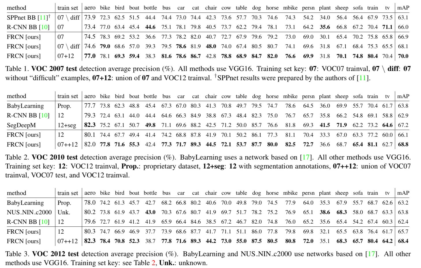
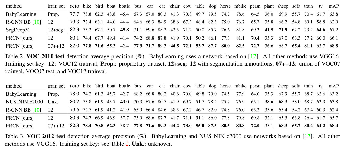
4.2. VOC 2010 and 2012 results

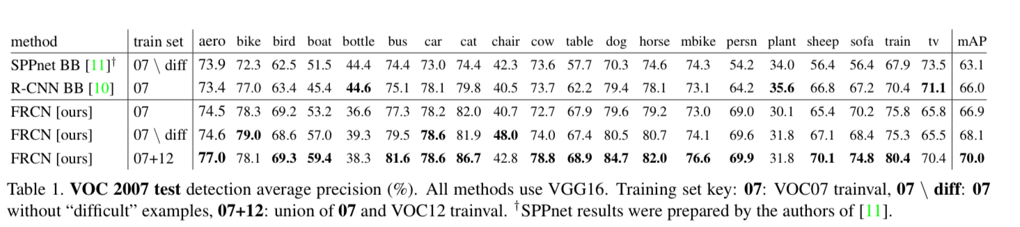
4.3. VOC 2007 results

4.4. Training and testing time

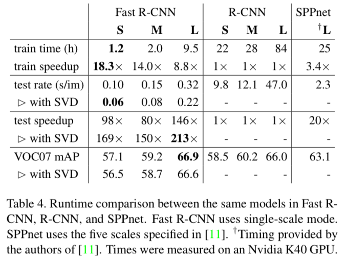
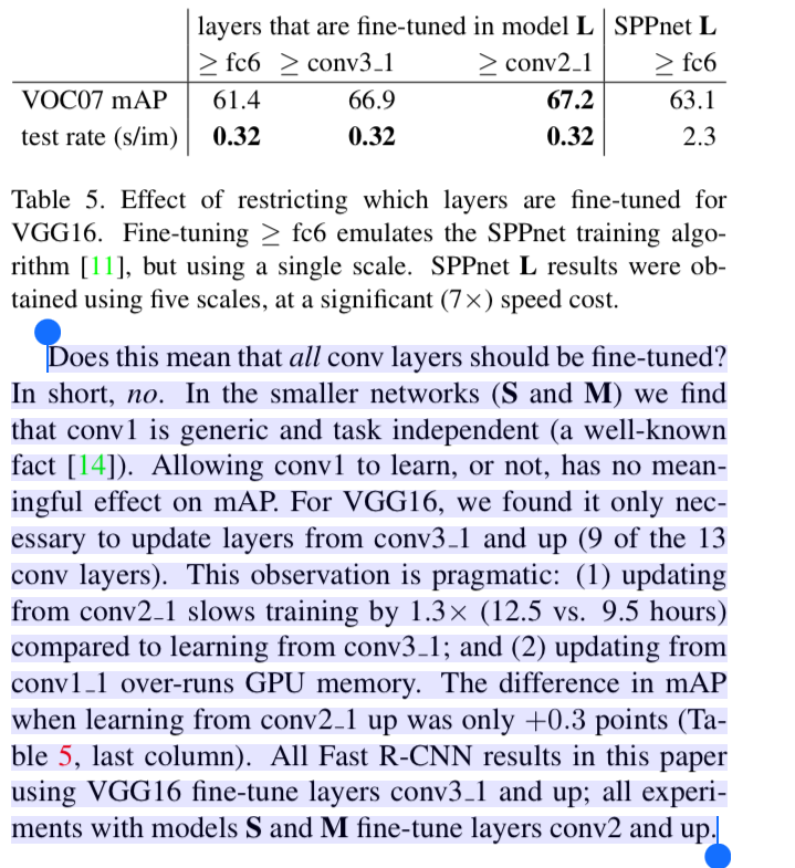
4.5. Which layer to fine-tune?

---

5. Design evaluation

(생략)

5.1. Does multi-task training help?

5.2. Scale invariance : to brute force of finesse?

5.3. Do we need more training data?

5.4. Do SVMs outperform softmax?

5.5. Are more proposals always better?

5.6. Preliminary MS COCO results

---

6. Conclusion

• 이 논문에서는 R-CNN 및 SPPnet에 대한 깔끔하고 빠른 update인 Fast R-CNN을 제안했다.
  특히 sparse object proposal은 detector quality를 향상시킬 수 있음을 보였다.
  이전에는 시간적으로 부담이 되어 연구하기 어려웠던 문제가 Fast R-CNN을 통해 실용적으로 되었다.
  물론 sparse proposal만큼 dense boxes가 허용되는 아직 발견되지 못한 기술들이 있겠지만,
  이러한 방법이 개발된다면 object detection을 더욱 가속화하는 데 도움이 될 것이다.

---

R-CNN에서 개선된 점

• R-CNN :
  만약 2k개의 region proposal을 생성해야 한다면,
  R-CNN에서는 selective search로 2k개의 region proposal을 만든 후,
  2k개 각각에 CNN을 적용해야 함.
  ➡️ 2k번 CNN을 해야 함.
  

• Fast R-CNN :
  만약 2k개의 region proposal을 생성해야 한다면,
  우선 한 image에 대해서 CNN을 한 번 적용한 후,
  selective search로 2개의 region proposal을 만든 후,
  2k개 각각의 RoI에 RoI pooling 해야 함.
  ➡️ 1번 CNN, 2k번 RoI pooling.