[2017 ICLR] OUTRAGEOUSLY LARGE NEURAL NETWORKS: THE SPARSELY-GATED MIXTURE-OF-EXPERTS LAYER
Paper Info.

Abstract
(문제 제기)
- information을 받아들이기 위한 neural network의 capacity는 그 network의 #parameter에 의해 제한된다.
per-example에 기반한 network의 일부분(parts)만 active하는 conditional computation은
computation의 proportional increase(비례적 증가) 없이 model capacity를 급격하게 증가시킬 수 있는 이론으로 제안되어 왔다.
하지만 실제로, significant algorithmic and performance challenges가 존재한다.
(아이디어)
- 이 연구에서, 우리는 이 challenges들을 해결하고 마침내 conditional computation의 promise(가능성)을 깨달았다.
우리는 only minor losses in computational efficiency on modern GPU clusters과 함께
model capacity에서 1000x improvements 이상을 달성할 수 있는 conditional computation을 제안한다.
우리는 thousands of fedd-forward sub-networks로 구성된 Sparsely-Gated Mixture-of-Experts layer (MoE)을 제안한다.
trainable gating network는 각 example에 사용할 experts들의 sparse combination을 결정한다.
(구체적 실험 결과)
- 우리는 vast quantitiles of(방대한 양의) training corpora에 포함된 knowledge를 흡수하기 위해 model capacity가 critical한
language modeling and machine translation tasks에 MoE를 적용했다.
우리는 최대 137 billion parameters를 가진 MoE를 stacked LSTM layers 사이에 convolutionally 적용한 model architecture를 제시한다.
Large language modeling and machine transloation benchmarks에서, 이 model들은 better results than SOTA at lower computational cost를 달성했다.
1. Introduction and Related Work
1.1 Conditional Computation
(conditional computation이 왜 등장했는가)
- training data and model size에 대한 scale exploiting(활용)은 DL의 성공에 중심이 되어왔다.
datasets이 충분히 클 때, NN의 capacity(#params) 증가는 much better prediction accuracy를 줄 수 있다.
불행히도, computing power의 발전과 distributed computation은 demand를 충족하기에 부족하다..
(conditional computation은 어떻게 발전해왔는가)
- a proportional increase(비례적 증가) in computational costs 없이 model capacity를 증가시키는 여러 형태의 conditional computation이 제안되어 왔다.
(이러한 방식에서는 large parts of network는 per-example로 active or inactive된다.
gating decisions은 binary or sparse and continuous일 수 있으며, stochastic and deterministic일 수도 있다.
gating decisions을 학습시키기 위한 RL and back-propagation들이 제안되어왔다.)
(이전 conditional computation은 어떤 문제가 있는가)
- 이러한 ideas들은 theory에서는 유망했지만, 현재까지 model capacity, training time, or model quality에서 massive improvements(대규모 개선)를 보여준 작업은 없었다.
우리는 이를 다음과 같은 challenges들의 combination에 기인한다고 본다:- 특히 GPU와 같은 modern computing devices는 branching보다는 arithmetic(산술 연산)에 훨씬 빠르다.
대부분의 앞선 연구들은 이 사실을 인식하고, 각 gating decision에서 network의 large chunks를 turning on/off하는 방법을 제안했다.
(내가 생각한 의미 해석:
GPU는 복잡한 조건문을 처리하는 것보다 단순한 수학적 계산을 수행하는 데 훨씬 효율적이기 때문에
기존 연구들은 network의 큰 부분을 한 번에 active하거나 inactive하는 방식으로 conditional computation을 계산했다)
(내 생각: 그러면 기존 방법들은 잘 한거 아닌가?) - Large batch size는 performance에 critical하다.
large batch는 parameter transfers and updates의 비용을 amortize(분산시킨다)한다.
conditional computation은 network의 conditionally active chunks를 위해 batch sizes를 줄인다. - network bandwidth는 bottleneck이 될 수 있다.
A cluster of GPUs는 inter-device network(장치간 network) bandwidth보다 천 배 이상의 computational power를 가질 수 있다.
(내가 생각한 의미 해석:
분산 컴퓨팅 환경에서 알고리즘의 계산 효율성을 높이려면 network badnwidth보다 computational capacity(계산 요구량)이 더 커야 한다.
GPU는 연산 능력은 뛰어나지만, 여러 GPU 사이의 네트워크 대역폭은 상대적으로 제한적이다.
따라서 효율적인 계산을 위해서는 GPU 내에서의 연산량을 늘리고, GPU 간 데이터 전송을 최소화해야 한다.
예를 들어, embedding layer는 계산량 자체는 크지 않지만, network 전송 부담이 커서 전체적인 성능 향상을 저해함
즉 computational capacity보다는 network bandwidth에 의해 #(example, param interactions)이 제한됨) - scheme에 따르면, per-chunk and/or per example에 대해 원하는 수준의 sparsity를 달성하기 위해 loss terms이 필요하다.
Bengio et al. (2015)는 세 가지 loss terms을 사용했다.
이러한 issues는 model quality and load-balancing에 영향을 미칠 수 있다. - model capacity는 very large data sets에 대해서 critical하다.
conditional computation에 대한 기존의 literature는 최대 600,000 images를 포함하는 relatively small image recognition data sets을 다루고 있다.
이러한 images의 labels이 수백만, 수십억 개의 parameter를 가진 model을 적절히 train시키기에 sufficient signal을 제공한다고 생각하기는 어렵다.
- 특히 GPU와 같은 modern computing devices는 branching보다는 arithmetic(산술 연산)에 훨씬 빠르다.
- 이 연구에서, 처음으로 위에 언급한 모든 challenges를 해결하고, 마침내 conditional computation의 가능성을 실현했다.
우리는 model capacity에서 only minor losses computational efficiency와 함께 1000x 이상의 improvements를 얻었으며,
public language modeling and translation data sets에 대해서 SOTA를 크게 향상시켰다.
1.2 OUR APPROACH: THE SPARSELY-GATED MIXTURE-OF-EXPERTS LAYER
-
conditional computation에 대한 우리의 approach는
a new type of general purpose neural network component를 추가하는 것이다:a Sparsely-Gated Mixture-of-Experts Layer (MoE). -
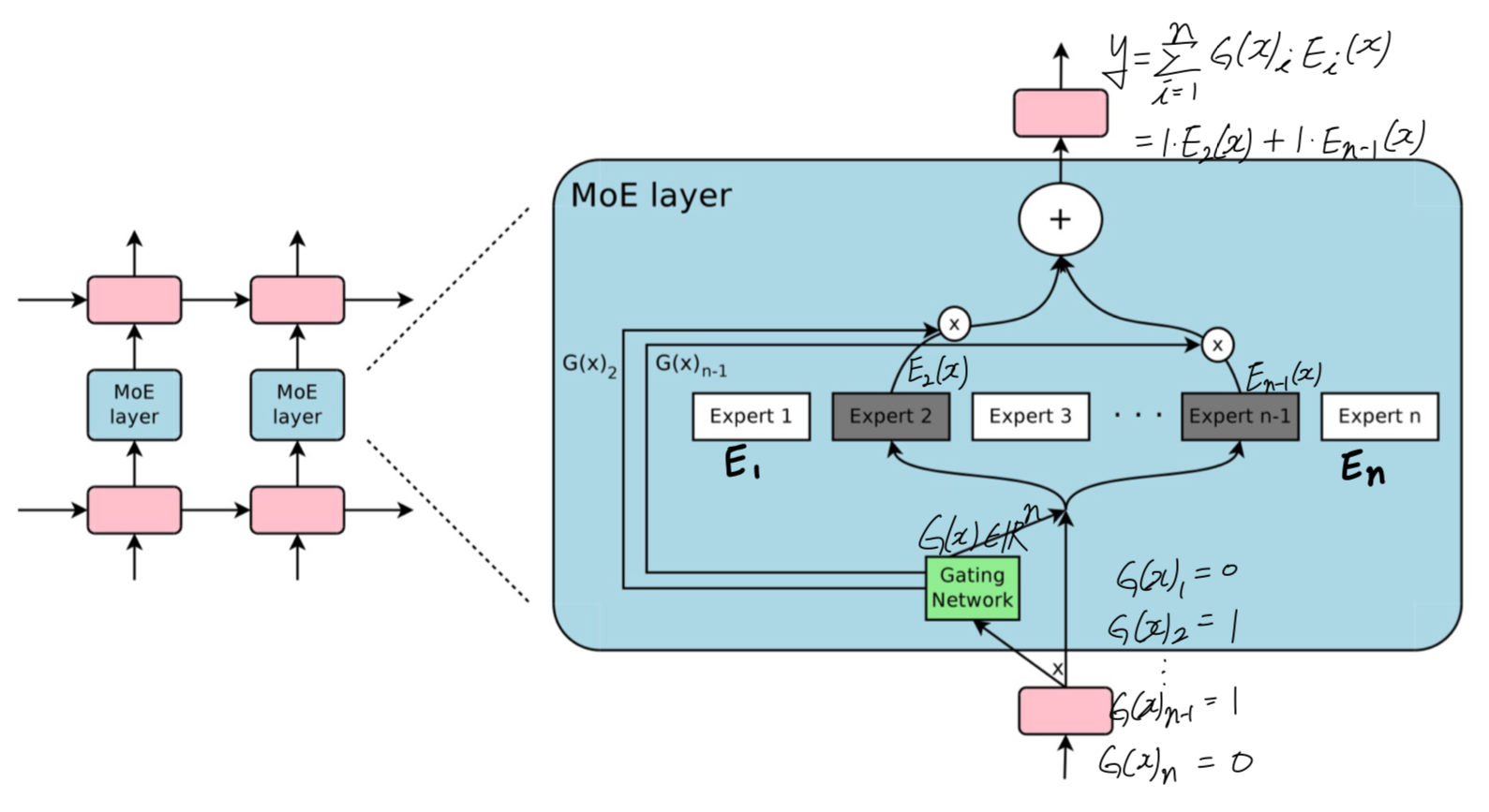
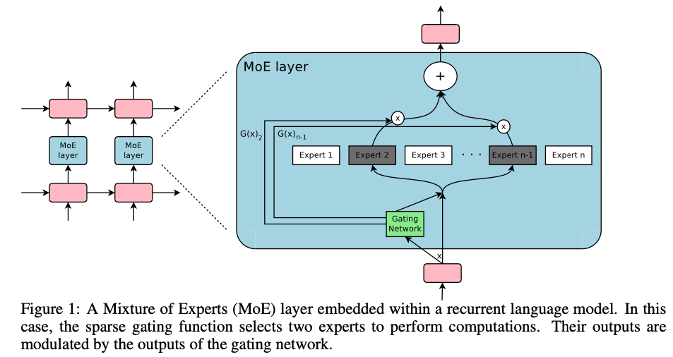
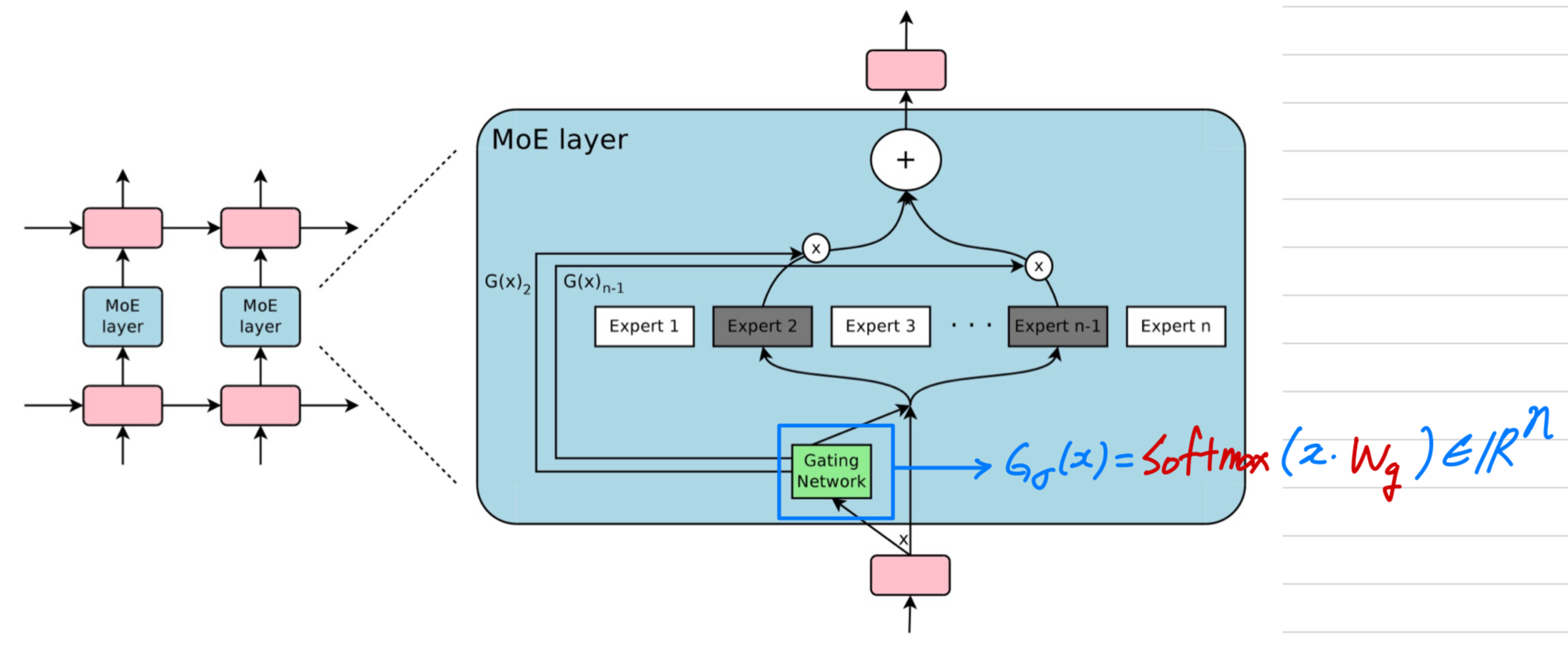
MoE layer는 많은 experts로 구성되어 있고,
각 expert는 a simple feed-forward neural network이며,
trainable gating network가 each input을 process하기 위한 experts의 a sparse combination을 선택한다. (Figure 1)
network의 모든 parts는 back-propagation에 의해 jointly trained된다.
 제안된 기술은 generic하지만, 이 논문에서 우리는 language modeling and machine translation tasks에 초점을 맞춘다.
특히, 우리는 MoE를 stacked LSTM layers 사이에 MoE를 convolutionally 적용했다.
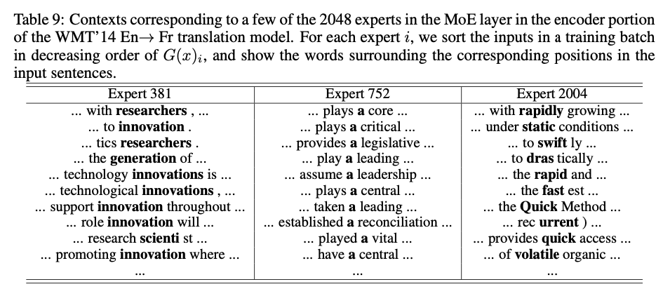
MoE는 각 text의 각 position에 대해 한 번 호출되며, 각 위치에서 잠재적으로 다른 experts의 combination을 선택한다.
다양한 experts들은 syntax and semantics를 기반으로 highly specialized되는 경향이 있다. (Appendix E Table 9)
1.3 RELATED WORK ON MIXTURES OF EXPERTS
-
the mixture-of-experts approach는 20년 이상 전에 도입된 이후, 많은 연구의 주제가 되어왔다.
다양한 유형의 expert architectures가 제안되었다.
예를 들어 SVM, Gaussian Processes, Dirichlet Processes, 그리고 deep networks 등이 있었다.
다른 연구들은 hierarchical structure, infinite nubmers of experts, 그리고 adding experts sequentially와 같은 다양한 experts configurations에 초점을 맞추었다.
위 연구들은 모두 top-level mixtures를 다루며, mixture of experts 자체가 전체 model로 사용되었다. -
Eigen et al.(2013)은 gating network를 deep model의 구성 요소로 사용하는 idea를 제안했다.
이러한 approach가 more powerful하다는 것을 직관적으로 알 수 있다.
complex problems은 각기 다른 experts를 필요로 하는 많은 sub-problems를 포함할 수 있기 때문이다.
그들은 또한 conclusion에서 sparsity 도입의 가능성을 언급하며, MoE를 computational computation을 위한 수단으로 전환할 가능성을 제시했다.
우리의 연구는 MoE를 general purpose neural network component로 사용하는 이러한 접근법에 기반하고 있다.
Eigen et al.(2013)은 두 개의 MoE를 쌓아 두 set의 gating decisions을 가능하게 한 반면, 우리의 MoE convolutional application은 text의 각 position에서 다른 gating decision을 내릴 수 있다.
우리는 또한 sparse gating을 구현했으며, 이를 통해 model capacity를 크게 증가시킬 수 있는 practical way로 활용할 수 있음을 입증했다.
2. THE STRUCTURE OF THE MIXTURE-OF-EXPERTS LAYER
-
MoE layer는 a set of "expert networks" 과
output으로 a sparse -deimensional vector를 갖는 "gating network" 로 구성된다. -
experts들은 자체의 parameters를 갖는 neural networks이다.
원칙적으로 experts들이 same sized inputs and produce the same-sized outputs을 생성하기만 하면 되지만,
이 논문에서의 initial investigations(초기 실험)에서는 feed-forward networks로 구성된 identical(동일한) architectures를 가지되, 각각의 parameters는 독립적인 경우로 제한했다.
(내가 이해한 내용: experts들은 내부 연산이 어떻게 되어 있든 same sized inputs and produce the same-sized outputs을 생성하기만 하면 된다.
근데 이 논문에서는 experts의 내부가 모두 동일한 FFN 구조를 갖도록 하였음.)
- input 가 주어졌을 때,
는 output of the gating network,
는 -th expert network
라고 하자.
MoE module의 output 는 다음과 같이 쓸 수 있다:
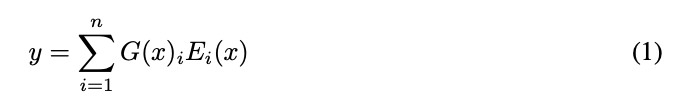 우리는 의 output의 sparsity에 기반하여 computation을 save할 수 있다.
이면, 를 계산할 필요가 없다.

우리의 experiments에서, 우리는 수천 개의 experts를 사용했지만, 각 example에 대해 evaluate해야 하는 expert는 소수에 불과하다.
만약 #experts가 매우 크면, 우리는 two-level hierarchical MoE를 사용함으로써 branching factor를 줄일 수 있다.
hierarchical MoE에서는, a primary gating network가 "experts"의 a sparse weighted combination을 선택하며,
각 "expert"는 자체 gating network를 가진 secondary mixture-of-experts로 구성된다.
(이후 내용에서는 ordinary MoEs(일반적인 MoEs)에 초점을 맞추고, hierarchical MoEs에 대한 details은 Appendix B에 제공한다.)
우리의 implementation은 다른 conditional computation model들과 연관되어 있다.
expert들이 simple weight matrices로 구성된 MoE는 (Cho & Bengio, 2014)에서 제안된 parameterized weight matrix와 유사하다.
expert들이 one hidden layer를 가지는 MoE는 (Bengio et al., 2015)에서 설명된 block-wise dropout과 유사하다.
이 경우 dropped-out layer는 fully-activated layers 사이에 위치한다.
궁금한 점:
그래서 이 저자들은 Expert마다 어떤 FFN을 구성했다는 것인가?
하나의 hidden layer를 갖는 FFN을 구성했다는 것 같은데...
2.1 GATING NETWORK
Softmax Gating
- Softmax Gating은 a simple choice of non-sparse gating function이고,
input에 trainable weight matrix 를 곱한 후, function을 적용하는 것이다.

Noisy Top-K Gating
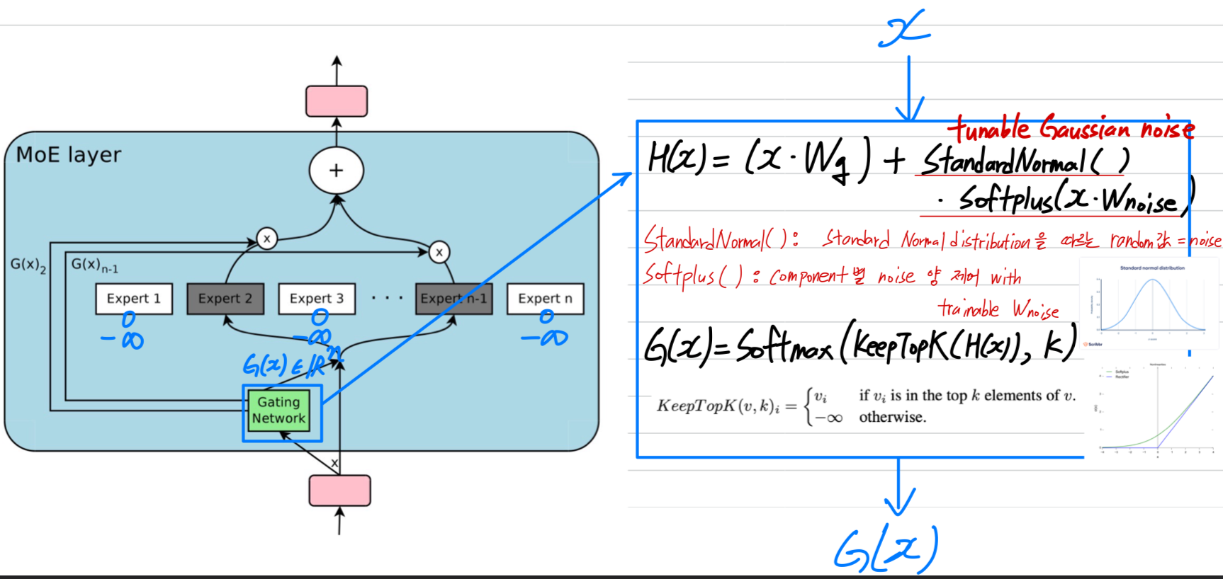
- 우리는 Softmax gating network에 two components를 추가했다: sparsity and noise.
softmax function에 넣기 전에, 우리는 tunable Gaussian noise를 추가한 뒤,
top values만 유지하고 나머지는 로 설정한다. (이는 softmax 이후 해당 gate values를 0으로 만들기 위함)
위에서 설명한 대로, 이 sparsity는 computation을 줄여줄 수 있다.
이 형태의 sparsity는 이론적으로 gating function의 output에서 discontinuities를 유발할 수 있지만, 실제 실험에서는 문제가 되는 경우를 관찰하지 못했다.
noise term은 load balancing에 도움이 되며, 이는 Appendix A에서 discussed.
각 componenet 별 noise의 양은 second trainable weight matrix 에 의해 제어된다.
(아래 그림 참고 : https://cameronrwolfe.substack.com/p/conditional-computation-the-birth)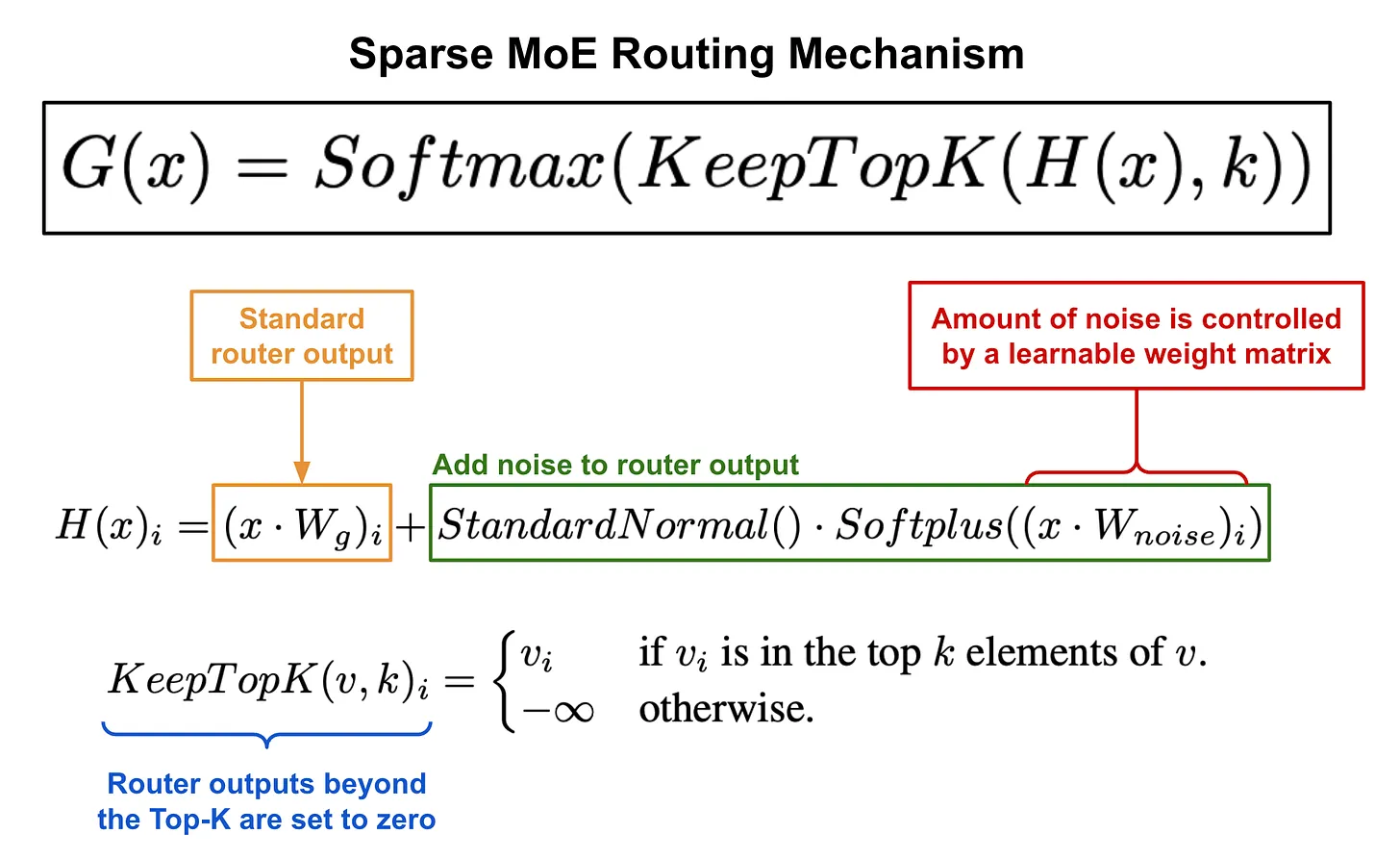
Training the Gating Network
- gating network는 model의 나머지 부분과 함께 simple back-propagation을 통해 train했다.
만약 로 설정하면, top experts에 대한 gate values는 gating network의 weights에 대해 nonzero derivatives(0이 아닌 기울기)를 갖게 된다.
이와 같은 occasionally-sensitive behavior(간헐적으로 민감한 동작)은 (Bengio et al., 2013)에서 noisy rectifiers에서 설명된 바 있다.
Gradients는 gating network를 통해 해당 input까지도 back-propagate된다.
우리의 방법은 (Bengio et al., 2015)과 다르다.
(Bengio et al., 2015)에서는 boolean gates를 사용하고, gating network를 학습시키기 위해 REINFORCE-style approach를 사용했다.
3. ADDRESSING PERFORMANCE CHALLENGES
3.1 THE SHRINKING BATCH PROBLEM
- 현대 CPUs and GPUs에서, large batch sizes는 computational efficiency를 위해 필수적이다.
이는 parameter loads and updates로 인한 overhead를 분산(amortiaze)시키기 위함이다.
만약 gating network가 각 example에 대해 experts 중 를 선택했다면,
batch size가 인 경우, 각 expert는 대략적으로 개의 sample을 받게 된다.
이로 인해 expert 수가 증가함에 따라 naive MoE implementation은 inefficient하게 된다. - 이 shrinking batch problem을 해결하기 위한 방법은 original batch size를 가능한 크게 만드는 것이다.
하지만, batch size는 forward pass와 backward pass 사이에 activations을 저장하는 데 필요한 memory에 제한을 받는 경향이 있다.
따라서 우리는 batch size를 증가심키기 위해 다음의 techniques을 제안한다.
Mixing Data Parallelism and Model Parallelism:
-
conventional distributed training setting에서,
서로 다른 devices에 multiple copies of the model이 존재하며,
이들은 서로 다른 batches of data를 asynchronously(비동기적으로) 처리하고,
parameter는 parameter servers를 통해 synchronized된다.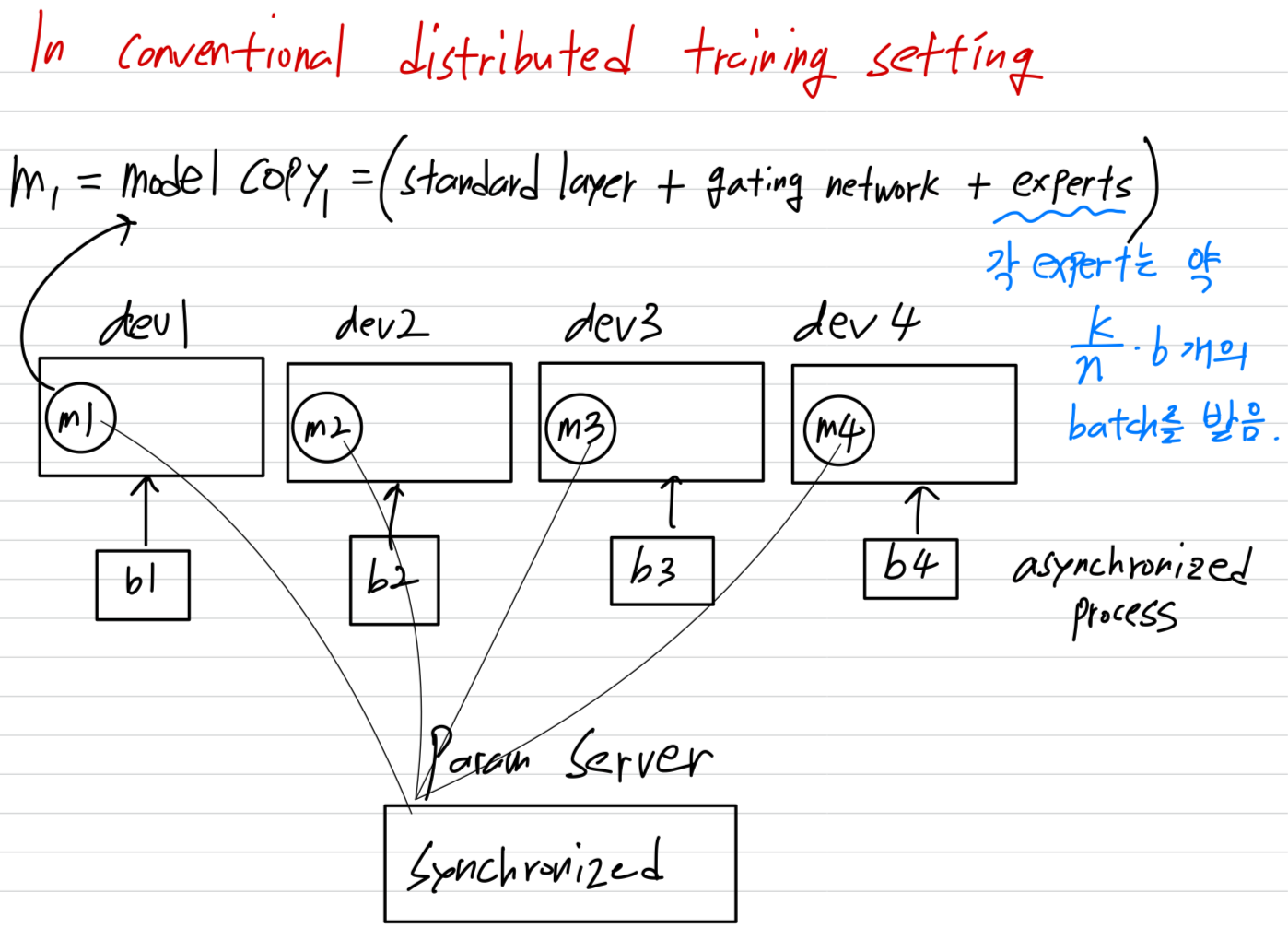 하지만 우리의 technique에서, 이 서로 다른 batches들이 synchronously(동기적으로) 실행되며, 이를 MoE layer에서 combined할 수 있다.
 -
우리는 model의 standard layers와 gating network를 기존의 data-parallel schemes에 따라 distribute하되,
each expert의 shared copy는 하나만 유지한다.
MoE layer의 each expert는 all of the data-parallel input batches로부터 관련된 examples들로 구성된 a combined batch를 받는다.
The same set of devices는 data-parallel replicas(복제본)(standard layers와 gating networks를 위해)으로도 동작하고,
model-parallel shards(각 experts의 subset을 hosting)로도 동작한다.
model이 개의 devcies에 distributed되고, 각 device가 size 인 batch를 처리한다고 가정하면,
각 expert는 대략 개의 examples로 이루어진 batch를 받는다.
이로 인해 expert batch size에서 배의 improvement를 달성한다.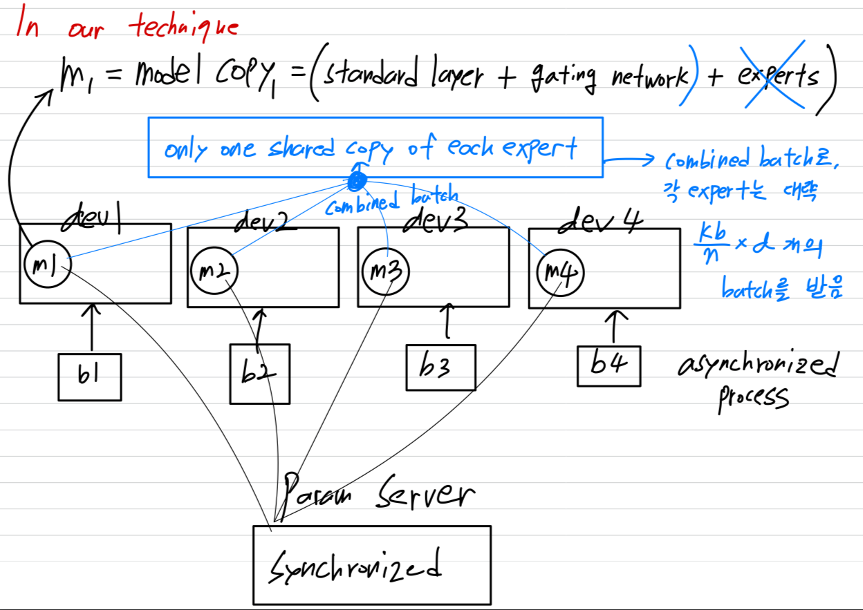
- 궁금한 점 : only one shared copy of each expert는 특정 device에 올려져 있겠지?

- 궁금한 점 : only one shared copy of each expert는 특정 device에 올려져 있겠지?
-
이 technique을 통해 #experts(and hence #params) = 를 증가시키기 위해 training cluster의 #devices = 를 proportionally(비례적으로) 증가시킬 수 있다.
 총 batch size는 증가하되, expert당 batch size는 일정하게 유지된다.(?)
또한, 각 device의 memory and bandwidth requirements 역시 일정하게 유지되며, step times과 model의 #params와 동일한 수의 training examples을 처리하는 데 걸리는 시간도 동일하게 유지된다.- 궁금한 점 : experts 복사본은 모든 개의 device마다 갖도록 하지 않고, only one shared copy로 떼어둔건 이해했다...
내 이해가 맞다면, 각 device에 experts가 올려져 있던 메모리 공간만큼의 batch size 증가만 가능한 것인가?
각 device에 experts가 올려져 있던 메모리 공간이 작았다면, 증가시킬 수 있는 총 batch size는 미미한거 아닌가?- NotebookLM 답변 :
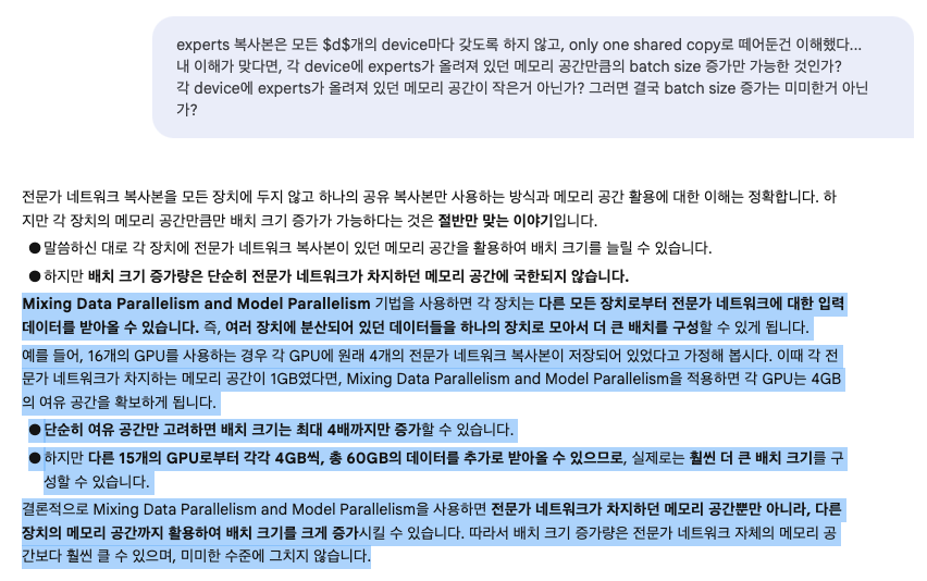
- NotebookLM 답변 :
- 궁금한 점 : experts 복사본은 모든 개의 device마다 갖도록 하지 않고, only one shared copy로 떼어둔건 이해했다...
- 우리는 trillion-word corpus로 trillion-parameter model을 학습시키는 것을 목표로 하고 있다.
이 논문을 작성하는 시점에는 우리의 system을 이 정도로 확장하지는 않았으나, 더 많은 HW를 추가하면 가능할 것으로 보인다.
Taking Advantage of Convolutionality:
- 우리의 language models에서, 우리는 previous layer의 각 time step에 동일한 MoE를 적용했다.
previous layer가 완료될 때까지 기다린 후, 모든 time steps을 one big batch로 묶어 MoE를 적용할 수 있다.
이렇게 하면 MoE layer에 대한 input batch의 size가 풀어진 time steps의 수만큼 증가한다.
Increasing Batch Size for a Recurrent MoE:
- skip
3.2 NETWORK BANDWIDTH (?)
-
distributed computing에서 또 다른 major performance concern은 network bandwidth이다.
experts들이 staionary(고정되어 있으며)하며 #gating parameters가 적기 때문에,
대부분의 communication은 expert의 input and output을 network를 통해 전송하는 것과 관련이 있다.
computational efficiency를 유지하려면, expert의 computation과 input and output 크기 비율이
computing device의 계산 대 network capacity 비율을 초과해야 한다.
GPU의 경우, 이 비율은 thousands to one(수천 대 1)일 수 있다. -
우리의 실험에서는 하나의 hidden layer에 수천 개의 RELU-activated units을 가진 expert를 사용한다.
expert의 weight matrices는 and 크기를 가지므로, 계산 대 입력 및 출력의 비율은 hidden layer의 크기와 같다.
편리하게도, 우리는 더 큰 hidden layer이나 더 많은 hidden layer를 사용하여 computational efficiency를 증가시킬 수 있다.
4. BALANCING EXPERT UTILIZATION
-
우리는 gating network가 항상 동일한 몇몇 experts에게 large weights를 부여하는 상태로 converge하는 경향이 있다는 것을 관찰했다.
이 imbalance는 self-reinforcing하며, favored(선호된) experts들이 더 빠르게 학습되기 때문에 gating network에 의해 더 자주 선태괸다.
Eigen et al.(2013)은 같은 현상을 설명하며, 이 local minimum을 피하기 위해 학습 초기에 hard constraint를 사용했다.
Bengio et al. (2015)는 각 gate의 batch-wise average에 대해 soft constraint를 포함했다. -
우리는 soft constraint approach를 취했다.
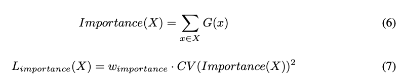
우리는 expert의 importance를 해당 expert의 gate value들의 batchwise sum으로 정의했다.
그리고 전체 model의 loss function에 추가의 loss 를 정의했다.
이 loss는 importance values의 the square of the coefficient of variation(변동 계수의 제곱)에 hand-tuned scaling factor 를 곱한 값이다.
이 추가의 loss는 모든 experts가 동일한 importance를 가지도록 유도한다.
-
이 loss function은 equal importance를 보장할 수 있지만, experts들이 여전히 매우 다른 수의 examples을 받을 수 있다.
예를 들어, 하나의 expert는 large weights를 가진 a few examples을 받는 반면, 다른 expert는 small weights를 가진 many examples을 받을 수 있다.
이는 distributed HW에서 memory and performance prlbmes을 일으킬 수 있다.
이 문제를 해결하기 위해 우리는 balanced loads를 보장하는 second loss function, 을 도입했다.
이 function의 정의와 experimental results는 Appendix A에 있다.
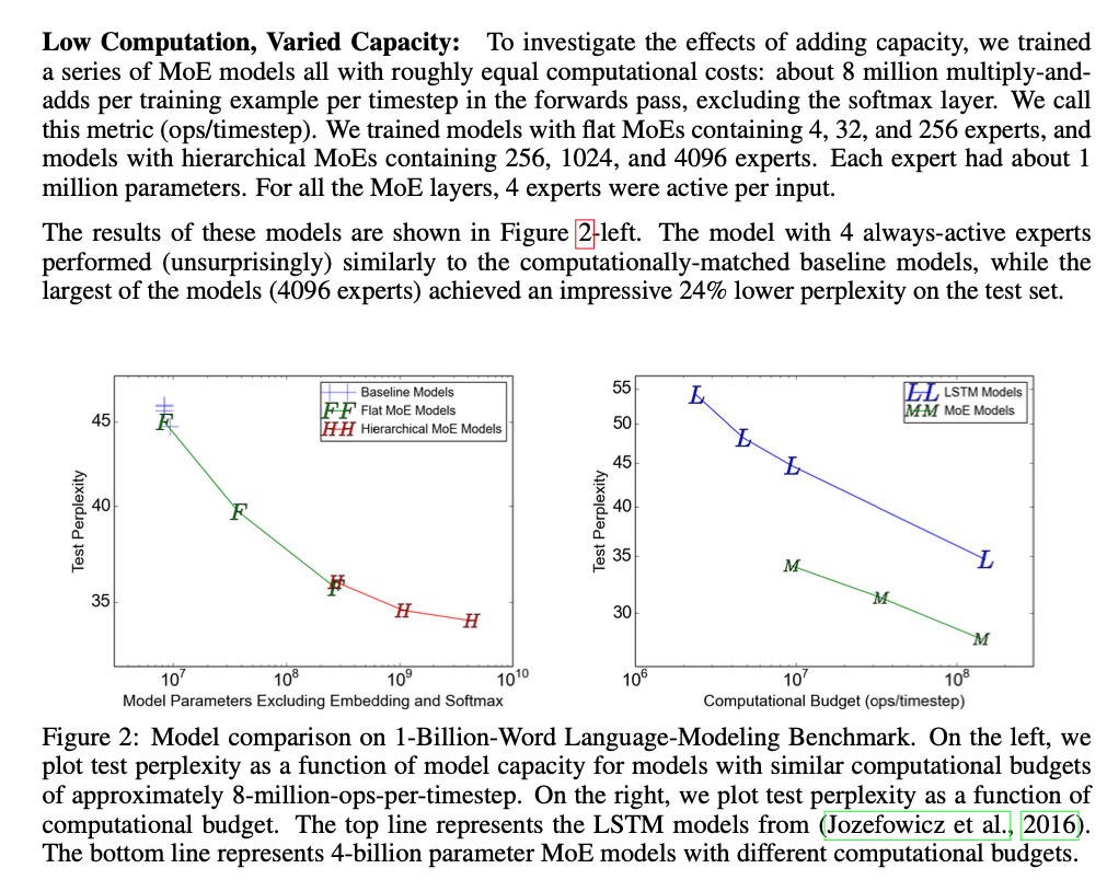
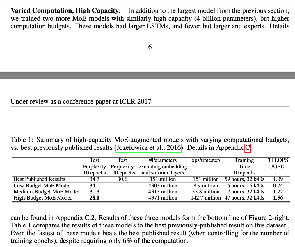
5. EXPERIMENTS